Last-Night Revision Sheet (DBMS)
How to Use This Guide
This guide assumes zero background. Each topic starts with an “Understand it first” explanation in plain words with a real-life comparison, then the exam-ready material (definitions, diagrams, examples, SQL), then common mistakes and “check yourself” questions. SQL examples use Oracle syntax (what your unit notes and the Ivan Bayross reference book use).
| syntax | (what your unit notes and the Ivan Bayross reference book use). | |
|---|---|---|
| Unit | Topic | Weightage |
| 1 | Database system architecture | 10 |
| 2 | Data models (ER model, integrity constraints) | 15 |
| 3 | Relational query languages (algebra, calculus, SQL) | 10 |
| 4 | Relational database design (FD, normalisation) | 15 |
| 5 | Query processing & optimisation | 10 |
| 6 | Transaction processing, concurrency, recovery, security | 15 |
| 7 | SQL concepts & PL/SQL | 25 |
Strategy: Unit 7 (SQL + PL/SQL) is a quarter of the paper — write queries by hand until it’s automatic. Units 2, 4 and 6 come next (15 each) and are very “pattern” based: ER diagrams, normalisation steps, serializability tests. Each unit ends with the questions your slides list as “asked in exam”.
One running example is used throughout the guide so you only learn the tables once:
STUDENT(RollNo, Name, Branch, Sem, SPI, City)
COURSE(CourseID, Title, Credits, DeptName)
ENROLL(RollNo, CourseID, Grade)
EMP(EmpNo, Ename, Job, Salary, DeptNo, MgrNo, HireDate)
DEPT(DeptNo, Dname, Location)
Database System Architecture
1.1 Basic definitions
Understand it first
Think of your college. It keeps information about thousands of students, courses, marks, fees. Where is it kept, and how does the office quickly answer “show all CSE students with SPI above 8”? A database is the organised storage, and a DBMS is the software that manages it — like a very smart, very strict librarian who stores data, finds it instantly, stops unauthorised people from seeing it, and makes sure two clerks updating the same record at the same time don’t mess it up.
Everyday DBMS you have used without noticing: the GTU/college result website, IRCTC train booking, your bank app, Instagram.
| Term | Meaning | Example | |
|---|---|---|---|
| Data | Raw facts that can be | recorded | “Maher”, 19, “CSE” |
| Information | Processed, meaningful data | “Maher is a 19-year-old CSE student” | |
| Database | A collection of logically data stored together | related | University student database |
| DBMS | Software to create, store, manage, retrieve and secure databases | Oracle, MySQL, SQL Server, PostgreSQL | |
| Database system | Database + DBMS software application programs + | + users | |
| Metadata | about table “Data data” — names, column types, constraints; stored in the dictionary / system catalog | data |
DBMS definition (exam): A Database Management System is a collection of inter-related data and a set of programs to access that data conveniently and efficiently, while ensuring security, integrity and concurrent access.
1.2 Historical perspective
| Period | Development |
|---|---|
| 1950s–60s | File processing systems on magnetic tape — sequential files; punched cards |
| 1960s | Hierarchical model (IBM IMS) and Network model (CODASYL/DBTG) on disks |
| 1970 | E. F. Codd (IBM) proposes the relational model |
| 1970s–80s | System R (IBM) and Ingres prototypes; SQL becomes standard (ANSI 1986); Oracle, DB2 released |
| 1980s–90s | Object-oriented and object-relational databases; client-server; parallel/distributed DBs |
| 2000s–now | Web-scale data, XML, data warehousing, NoSQL (MongoDB, Cassandra), cloud databases, Big Data |
1.3 File system vs DBMS
Understand it first
Before DBMS, each department kept its own files (like separate Excel sheets). The accounts office had a fees file with your address; the exam office had another file with your address. When you moved house, one office updated it and the other didn’t. Now which address is right? Every problem in the table below comes from this “separate files” approach.
Before DBMS, organisations stored data in separate files each managed by its own
program. This caused problems — and those problems are exactly the advantages of a DBMS.
| Problem in file system | How DBMS solves it |
|---|---|
| Data redundancy — same data stored in many files | Centralised storage, controlled redundancy |
| Data inconsistency — copies disagree (address updated in one file only) | One copy → consistent |
| Difficulty accessing data — new query needs a new program | Query language (SQL) |
| Data isolation — data scattered in different formats | Uniform structure |
| Integrity problems — constraints buried in code | Constraints declared once (CHECK, FK) |
| Atomicity problems — failure mid-transfer leaves partial update | Transactions are all-or-nothing |
| Concurrent-access anomalies — two users update simultaneously | Concurrency control (locking) |
| Security problems — hard to restrict who sees what | Users, roles, GRANT/REVOKE |
| No backup/recovery | Automatic backup and recovery |
Advantages of DBMS (list for 7 marks)
- Controls redundancy. 2. Removes inconsistency. 3. Data sharing among many
users/applications. 4. Enforces integrity constraints. 5. Security & authorisation. 6. Backup & recovery. 7. Concurrency control. 8. Data independence. 9. Standards enforcement. 10. Easy querying via SQL. 11. Reduced application development time.
Disadvantages of DBMS
High cost (software, hardware, staff); complexity; large size; performance overhead for small applications; a single failure can affect everyone (centralisation).
Applications of DBMS
Banking (accounts, transactions), airlines/railways (reservations), universities (registration, results), telecom (call records), e-commerce (orders, inventory), HR/payroll, hospitals (patient records), social media, government (Aadhaar, tax).
1.4 Three-level ANSI/SPARC architecture
Understand it first
Different people need different things from the same database:
a student only needs to see their own marks,
the designer needs to know every table and relationship,
the system needs to know exactly which disk block each record is in.
So the database is described at three levels, each hiding the details of the level below. Think of a building: visitors see only the rooms they’re allowed into (external), the
architect’s plan shows all rooms and how they connect (conceptual), and the engineer’s drawings show pipes, wires and foundations (internal).
The ANSI/SPARC committee proposed separating the user’s view from physical storage using three levels (schemas):
User 1
User 2
User 3
View 1
View 2
View 3
EXTERNAL LEVEL
Conceptual schema
CONCEPTUAL LEVEL
(what data, relationships, constraints)
Internal schema
INTERNAL LEVEL
(how data is stored: files, indexes)
Stored database
Three-level ANSI/SPARC architecture
| Level | Describes | Who uses it | Example |
|---|---|---|---|
| Internal / physical | How data is actually stored: files, record layout, indexes, compression, block size | DBA, system designers | STUDENT stored as a B+ tree file indexed on RollNo |
| Conceptual / logical | What data is stored and relationships — all entities, attributes, constraints for the whole database | DBA, designers | STUDENT(RollNo INT PK, Name VARCHAR2(30), SPI NUMBER(4,2)) |
| External / view | The part of the database relevant to a particular user group; hides the rest | End users, application programs | Accounts clerk sees only RollNo, Name, FeesDue |
1.5 Data abstraction
Data abstraction = hiding the complex storage details from users and showing only what they need. The three levels above are the three levels of abstraction: physical, logical, view.
Analogy: A car. Driver sees steering, pedals (view). Mechanic knows the engine design (logical). Manufacturer knows every bolt and metal grade (physical).
Schema vs instance: Schema = the overall design/structure of the database (rarely changes) — like a class/variable type. Instance = the data stored at a particular moment (changes constantly) — like an object/variable’s value.
1.6 Mappings and data independence
Understand it first
Data independence means “you can change one level without breaking the level above it”. Example: the DBA moves the database to a faster SSD and adds an index (internal change). Students’ apps keep working exactly the same — that’s physical independence. If the designer adds an Email column to STUDENT (conceptual change) and the old fee-payment app still works because its view didn’t change — that’s logical independence.
Mapping = the correspondence between two levels.
External/conceptual mapping — how each view’s fields correspond to the conceptual schema.
Conceptual/internal mapping — how conceptual records/fields are stored physically.
Data independence = the ability to change the schema at one level without having to change the schema at the next higher level.
| the schema at the next | higher level. | |
|---|---|---|
| Type | Meaning | Example change that should NOT affect higher level |
| Physical data independence | Change internal schema without changing conceptual schema | Add an index, move files to SSD, change file organisation |
| Logical data independence | Change conceptual schema without changing external schemas/applications | Add a new column Email to STUDENT; split a table |
Logical data independence is harder to achieve, because applications depend on the logical structure. Only the mapping is updated when a level changes.
1.7 Database users and the DBA
| User type | Description |
|---|---|
| Naive / parametric end users | Use ready-made application interfaces (ATM, ticket booking clerk) |
| Casual / sophisticated users | Write ad-hoc queries in SQL (analysts, scientists) |
| Application programmers | Write programs (Java/Python with embedded SQL) that access the DB |
| Specialised users | Write special DB applications (CAD, expert systems, multimedia) |
| Database designers | ER Decide the structure: tables, constraints, model |
| DBA (Database Administrator) | Has central control over data and programs |
Roles / functions / duties of the DBA
-
Schema definition — creates the conceptual schema using DDL.
-
Storage structure and access-method definition — decides physical organisation and indexes.
-
Schema and physical organisation modification — tunes as needs change.
-
Granting authorisation — creates users, GRANT/REVOKE privileges.
-
Routine maintenance — periodic backups, ensuring enough disk space, monitoring performance.
-
Recovery — restores the database after failures.
-
Integrity constraint specification and security policy.
-
Performance tuning, upgrades, liaison with users.
1.8 Database system architecture (overall structure)
 Naive users App programmers Sophisticated users DBA
 (app UI) (app programs) (query tools) (admin tools)
 │ │ │ │
 └─── application interfaces ── app programs ── query tools ── admin tools
 │
 ┌───────────────── QUERY PROCESSOR ───────────────────┐
 │ DDL interpreter DML compiler & organiser │
 │ (+ embedded DML precompiler) Query evaluation engine │
 └──────────────────────────┬──────────────────────────┘
 ┌───────────────── STORAGE MANAGER ───────────────────┐
 │ Authorization & integrity mgr Transaction mgr │
 │ File manager Buffer manager │
 └──────────────────────────┬──────────────────────────┘
 DISK STORAGE: data files, data dictionary, indices, statistical data
Query processor components
DDL interpreter — interprets DDL statements and records definitions in the data dictionary. DML compiler — translates DML (SQL) into a low-level query evaluation plan; also does query optimisation (picks the cheapest plan).
Embedded DML pre-compiler — converts SQL embedded in host-language programs into procedure calls.
Query evaluation engine — executes the low-level instructions.
Storage manager components
Authorization & integrity manager — checks constraints and user permissions.
Transaction manager — ensures consistency despite failures (atomicity) and concurrency. File manager — allocates disk space and data structures.
Buffer manager — moves data between disk and main memory (cache).
Disk storage: data files (the database itself), data dictionary (metadata), indices (fast access), statistical data (used by the optimiser).
1.9 Database languages
| Language | Purpose | Commands |
|---|---|---|
| DDL — Data Definition Language | Define/modify structure (schema) | CREATE, ALTER, DROP, TRUNCATE, RENAME |
| DML — Data Manipulation Language | Access and modify data | SELECT, INSERT, UPDATE, DELETE |
| DCL — Data Control Language | Permissions | GRANT, REVOKE |
| TCL — Transaction Control Language | Manage transactions | COMMIT, ROLLBACK, SAVEPOINT |
DML types: procedural (user says what data and how to get it — relational algebra) and declarative/non-procedural (user says only what — SQL, relational calculus).
Unit 1 — Questions asked in exam
-
List and explain the advantages of DBMS over file-based systems (or disadvantages of file systems).
-
Draw and explain the 3-level (ANSI/SPARC) architecture of DBMS.
-
Explain data abstraction and data independence (physical vs logical).
-
List and explain types of database users.
-
List and explain duties of the DBA.
-
Explain the overall DBMS (database system) architecture with a block diagram.
-
Differentiate DDL and DML; schema and instance.
Unit 1 — Check yourself
- Name three problems of the file system. 2. Which level of the 3-level architecture describes indexes? 3. Adding a column without changing users’ views is which
independence? 4. Two duties of a DBA.
Answers: 1) Redundancy, inconsistency, concurrent-access anomalies (also isolation, integrity,
atomicity, security). 2) Internal. 3) Logical. 4) Schema definition, granting authorisation (also
backup/recovery, tuning).
Data Models
A data model is a collection of concepts for describing data, relationships between data, semantics and constraints. Database design is the process of designing, developing and maintaining the database; the ER model is used for the first (conceptual) design step.
2.1 The Entity–Relationship (E-R) model
Understand it first
Before building tables, designers draw a picture of the data: what “things” exist (students, courses), what we store about them (name, credits), and how they’re connected (a student enrolls in a course). This picture is the E-R diagram. It’s like an architect’s sketch before construction — easy to discuss and fix before any table is created. Later, the diagram is converted into tables using fixed rules (section 2.8).
Proposed by Peter Chen (1976). An E-R diagram is a graphical (pictorial) representation of the database using symbols.
Basic concepts
Entity: a real-world object distinguishable from others — a particular student “Maher”, a particular course “DBMS”.
Entity set: a set of entities of the same type — all students. (Drawn as a rectangle.) Attribute: a property of an entity — RollNo, Name. (Drawn as an ellipse.)
Domain / value set: set of allowed values of an attribute — SPI ∈ [0, 10].
Relationship: an association among entities — Maher enrolls in DBMS.
Relationship set: a set of relationships of the same type — ENROLLS. (Drawn as a diamond.) A relationship can have its own attributes (Grade on ENROLLS).
Degree of a relationship: number of entity sets participating — unary/recursive (1: EMPLOYEE manages EMPLOYEE), binary (2, most common), ternary (3: SUPPLIER supplies PART to PROJECT).
ER notation (Chen)
| Symbol | Meaning |
|---|---|
| Rectangle | Strong entity set |
| Double rectangle | Weak entity set |
| Ellipse | Attribute |
| Ellipse with underlined name | Key (primary key) attribute |
| Double ellipse | Multivalued attribute |
| Dashed ellipse | Derived attribute |
| Ellipse connected to smaller ellipses | Composite attribute |
| Diamond | Relationship set |
| Double diamond | Identifying relationship (for weak entity) |
| Single line | Partial participation |
| Double line | Total participation |
| Arrow (→) towards entity | “One” side of cardinality |
| ISA Triangle labelled | Specialisation / generalisation |
Discriminator (partial key) of a weak entity
Dashed underline
2.2 Types of attributes
| Type | Meaning | Example |
|---|---|---|
| Simple (atomic) | Cannot be divided | RollNo, Age |
| Composite | Can be divided into sub-parts | Name → First, Middle, Last; Address → Street, City, Pin |
| Single-valued | One value per entity | DOB |
| Multivalued | Many values per entity (double ellipse) | PhoneNo, Email |
| Stored | Stored in the DB | DOB |
| Derived | Computed from others (dashed ellipse) | Age (from DOB), TotalMarks |
| Key attribute | an Uniquely identifies entity (underlined) | RollNo |
| Null-valued | Value may be unknown/not applicable | MiddleName |
Complex
Composite + multivalued
Multiple addresses each with street/city
combined
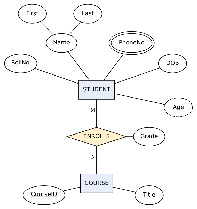
ER diagram: key attribute underlined, Name composite, PhoneNo multivalued (double ellipse), Age derived (dashed),
ENROLLS is an M:N relationship with attribute Grade
2.3 Mapping cardinality (cardinality ratio)
Understand it first
Cardinality answers: “how many of B can one A be connected to, and vice versa?”
One person has one passport, one passport belongs to one person → 1:1.
One department has many employees, each employee is in one department → 1:N. One student takes many courses, one course has many students → M:N.
The number of entities to which another entity can be associated via a relationship set (binary R between A and B):
| Cardinality | Meaning | Example |
|---|---|---|
| One-to-one (1:1) | An A relates to at most one B, and vice versa | PERSON — has — PASSPORT |
| One-to-many (1:N) | An A relates to many B’s; a B relates to at most one A | DEPARTMENT — has — EMPLOYEE |
| Many-to-one (N:1) | Many A’s to one B | EMPLOYEE — works in — DEPARTMENT |
| Many-to-many (M:N) | Many to many | STUDENT — enrolls — COURSE |
 [DEPARTMENT] 1 ───< has >─── N [EMPLOYEE]
 [STUDENT] M ───< enrolls >─── N [COURSE]
Participation constraints
Total participation (double line): every entity must participate. Every LOAN must belong to some CUSTOMER.
Partial participation (single line): some entities may not participate. Not every CUSTOMER has a LOAN.
2.4 Keys (needed for ER and relational model)
Understand it first
A key is whatever lets you point at exactly one row. Your name isn’t a key (two students can be named Raj), but your enrolment number is. Note the chain: every candidate key is a super key with nothing extra; the primary key is the one candidate key we choose; the remaining candidates are alternate keys.
| Key | Definition | Example in STUDENT | ||
|---|---|---|---|---|
| Super Candidate Primary Alternate Foreign Composite Partial | key key key key key key key / discriminator | Any set of attributes that uniquely identifies a tuple Minimal super key (no proper subset is a super key) The candidate key chosen by the designer; NOT NULL + unique Candidate keys not chosen as primary Attribute in one table that refers to the primary key of another Key with more than one attribute Attribute that identifies a weak entity only together with owner’s key | {RollNo}, {RollNo, Name}, {EnrollNo, Branch} {RollNo}, {EnrollNo} RollNo EnrollNo ENROLL.RollNo → STUDENT.RollNo {RollNo, CourseID} in PaymentNo | |
| Every | UNDERSTAND | candidate key is a super key; Weak entity sets IT | not every super key is a candidate | key. |
Understand it first
Some things can’t be identified on their own. “Payment number 1” means nothing alone — payment 1 of which loan? A payment only makes sense together with its loan. Such an entity is weak; the loan is its owner. Similarly, an employee’s dependent “Riya” is identified only together with the employee.
A weak entity set does not have a primary key of its own; it depends on a strong
(owner/identifying) entity set.
Drawn as a double rectangle; linked to the owner via a double diamond (identifying relationship) with total participation (double line).
Its discriminator (partial key) is underlined with a dashed line.
Primary key of weak entity = primary key of owner + discriminator.
 [ LOAN ] ══<< loan_payment >>══ [[ PAYMENT ]]
 (LoanNo) (PaymentNo - - -) (Amount) (Date)
 PK(PAYMENT) = {LoanNo, PaymentNo}
Other examples: DEPENDENT of EMPLOYEE (identified by EmpNo + DependentName); ROOM of BUILDING.
| Strong entity | Weak entity |
|---|---|
| Has its own primary key | No primary key; has a discriminator |
| Rectangle | Double rectangle |
| Independent existence | Existence depends on owner |
| Relationship: single diamond | Identifying relationship: double diamond |
2.6 Extended E-R (EER) features
Understand it first
Sometimes entities form a family: every faculty member and every staff member is an employee, sharing name, salary, etc., but each has extra details. EER features let the diagram show this “is-a” relationship (Faculty is an Employee), exactly like inheritance in Java.
Specialisation (top-down)
Dividing a higher-level entity set into lower-level sub-groups with distinguishing features. EMPLOYEE → {FACULTY, STAFF}. Subclasses inherit all attributes and relationships of the superclass and add their own.
Generalisation (bottom-up)
Combining several entity sets with common features into a higher-level entity set. CAR and TRUCK → VEHICLE. It is the reverse of specialisation.
 [ PERSON ] (Id, Name, Address)
 |
 /ISA\
 / \
 [ EMPLOYEE ] [ CUSTOMER ]
 (Salary) (CreditRating)
Constraints on specialisation / generalisation
- Membership condition:
Condition/predicate-defined — membership decided by an attribute value (Job = ‘Faculty’).
User-defined — assigned manually by the user.
- Disjointness:
Disjoint — an entity belongs to at most one subclass (a person is either Student or Faculty). Write “disjoint” near ISA.
Overlapping — may belong to more than one (a person can be both Employee and Customer).
- Completeness:
Total — every superclass entity must belong to some subclass (double line).
Partial — some may belong to none (single line).
Aggregation
ER cannot express a relationship between a relationship and an entity. Aggregation treats a relationship set (with its entities) as a single higher-level abstract entity, which can then participate in another relationship.
Example: EMPLOYEE works-on PROJECT; this whole works-on relationship is monitored-by a MANAGER.
 ┌────────────────────────────────────────┐
 │ [EMPLOYEE]──<works_on>──[PROJECT] │ ← aggregated (boxed)
 └────────────────┬───────────────────────┘
 <monitors>
 │
 [MANAGER]
2.7 E-R diagram of a Hospital Management System (case study)
Entities and attributes
PATIENT (PatientID, Name, Age, Gender, Address{Street, City}, {PhoneNo})
DOCTOR (DoctorID, Name, Specialisation, Salary)
WARD (WardNo, WardType, Capacity)
TEST (TestID, TestName, Cost)
NURSE (NurseID, Name, Shift)
BILL — weak entity of PATIENT (BillNo partial key, Amount, Date)
Relationships
DOCTOR treats PATIENT — M:N, attribute Date.
PATIENT admitted_in WARD — N:1, attributes AdmitDate, DischargeDate.
NURSE assigned_to WARD — N:1.
PATIENT undergoes TEST — M:N, attribute Result.
PATIENT has BILL — identifying relationship (double diamond), total participation of BILL.
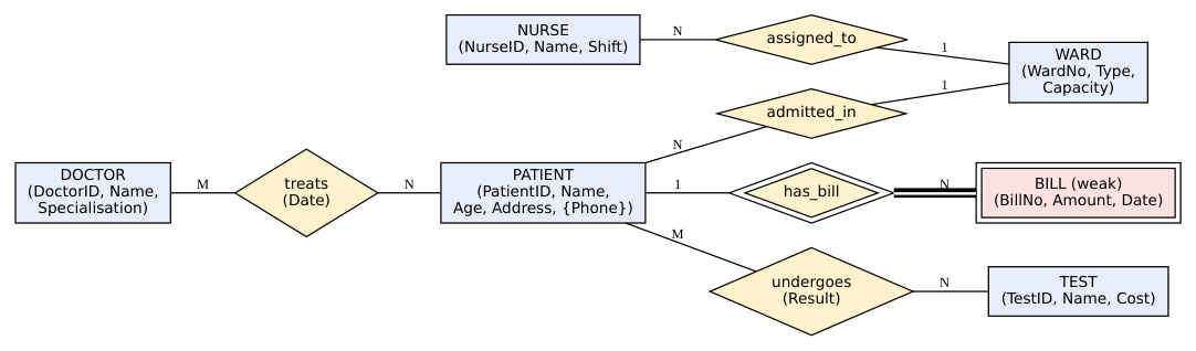
ER diagram of the Hospital Management System (BILL is a weak entity; has_bill is its identifying relationship)
| Reduction of an E-R diagram | to relational schema | (tables) | |
|---|---|---|---|
| ER construct | Rule | Example | |
| Strong entity | One table; simple attributes become columns; key → PK | STUDENT(RollNo, | Name, DOB) |
| Composite attribute | Keep only its component attributes | Name → FirstName, columns | LastName |
| Multivalued attribute | Separate table: (PK of entity, attribute); both form the PK | STUDENT_PHONE(RollNo, PhoneNo) | |
| Derived attribute | Not stored (computed) | Age omitted | |
| Weak entity | Table with its attributes + PK of owner; PK = owner PK + discriminator; FK to owner | PAYMENT(LoanNo, Amount) | PaymentNo, |
| 1:1 relationship | Add PK of either side as FK in the other (prefer the total- participation side) | PERSON(.., PassportNo | FK) |
| 1:N relationship | Add PK of the “1” side as FK in the “N” side | EMPLOYEE(.., DeptNo | FK) |
| M:N relationship | Separate table with PKs of both sides (+ relationship attributes); PK = both FKs | ENROLL(RollNo, | CourseID, Grade) |
| Specialisation | (a) table for superclass + table per subclass with PK superclass PK; = or (b) only subclass tables with inherited attributes (if total & disjoint) | PERSON(Id,Name), Salary) | EMPLOYEE(Id, |
MONITORS(EmpID, ProjID, MgrID) Aggregation
Table for the relationship with the
aggregated relationship’s PK +
other entity’s PK
2.9 Database (data) models
| Model | Structure | Notes |
|---|---|---|
| Hierarchical | Tree: each child has one parent (1:N); records linked by pointers | IBM IMS; fast for hierarchical data, cannot represent M:N easily; insertion/deletion anomalies |
| Network | Graph: a record can have many parents; owner–member sets | CODASYL/DBTG; handles M:N; complex pointer navigation |
| Relational | Data in tables (relations) of rows and columns; relationships via keys | Codd 1970; simple, SQL, data independence; most widely used |
| Object-oriented | Data as objects with attributes + methods; classes, inheritance, encapsulation, object identity | Good for CAD, multimedia, complex data; ObjectDB, db4o |
| Object-relational | Relational + objects (user-defined types, inheritance) | Oracle, PostgreSQL |
| ER model | Conceptual model (entities, relationships) | Used for design, then mapped to relational |
Hierarchical: Network: Relational:
 Dept Dept Project EMP table DEPT table
 / \ \ / +----+--+ +--+-----+
 Emp Emp Emp |E1 |10| |10|Sales|
 +----+--+ +--+-----+
2.10 Integrity constraints
Understand it first
Constraints are rules the DBMS enforces automatically, so wrong data can never enter: SPI can’t be 15, two students can’t share a roll number, you can’t enroll a student who doesn’t exist.
Rules that ensure the data in the database stays accurate and consistent.
-
Domain constraint — each attribute’s value must come from its domain (data type, range). SPI NUMBER(4,2) CHECK (SPI BETWEEN 0 AND 10) .
-
Entity integrity constraint — the primary key cannot be NULL (and must be unique).
-
Referential integrity constraint — a foreign key value must either match an existing primary-key value in the referenced table or be NULL. You cannot enroll RollNo 999 if no
student 999 exists. On delete of the parent: RESTRICT, CASCADE, SET NULL.
-
Key constraint — candidate key values must be unique (UNIQUE).
-
NOT NULL constraint — a column must always have a value.
-
CHECK constraint — arbitrary condition on a row ( Salary > 0 ).
-
Assertions / triggers — complex constraints spanning tables (Unit 7).
Data manipulation operations on the relational model: insert, delete, update, retrieve (select) — each must preserve the integrity constraints (an insert can violate
domain/key/entity/referential constraints; a delete can violate referential integrity; an update can violate any).
Data security vs data integrity: integrity = correctness/consistency of data (constraints). Security = protection of data from unauthorised access (users, privileges, encryption).
Unit 2 — Questions asked in exam
-
Explain the components/symbols of an E-R diagram. Types of attributes with examples.
-
Explain mapping cardinalities and participation constraints.
-
What is a weak entity set? Explain with example.
-
Explain specialisation, generalisation and their constraints; aggregation.
-
Draw an E-R diagram for a hospital / library / university / bank system.
-
Explain the reduction of E-R diagram to tables.
-
Compare hierarchical, network, relational and object-oriented models.
-
What is a constraint? Explain types of integrity constraints.
Unit 2 — Common mistakes
Putting the FK on the “1” side of a 1:N relationship (it goes on the N side).
Forgetting a separate table for an M:N relationship or a multivalued attribute.
Weak entity drawn with a single rectangle/diamond.
Unit 2 — Check yourself
- Symbol for a derived attribute? 2. PK of weak entity PAYMENT (discriminator
PaymentNo) owned by LOAN (LoanNo)? 3. How is an M:N relationship converted to tables?
Answers: 1) Dashed ellipse. 2) (LoanNo, PaymentNo). 3) A new table with the PKs of both entities (+ relationship attributes).
Relational Query Languages
3.1 Structure of relational databases
| Formal term | Informal term | Meaning |
|---|---|---|
| Relation | Table | Set of tuples with the same attributes |
| Tuple | Row / record | One entity’s data |
| Attribute | Column / field | A named property |
| Domain | Data type / allowed values | Set of permitted values |
| Degree (arity) | Number of columns | STUDENT(RollNo, Name, Branch, Sem, SPI) has degree 5 |
| Cardinality | Number of rows | 60 students → cardinality 60 |
| Relation schema | Table definition | STUDENT(RollNo, Name, Branch, Sem, SPI) |
| Relation instance | Table contents at a moment |
Properties of a relation: no duplicate tuples; order of tuples and attributes is irrelevant; each value is atomic (single); each attribute has a distinct name.
Keys (super, candidate, primary, alternate, foreign, composite) — see Unit 2.4.
3.2 Relational Algebra
Understand it first
Relational algebra is a small set of operations on tables that produce new tables — like +, −, × for numbers, but for tables. You combine them to answer questions. Every SQL query you write is internally converted into relational algebra so the DBMS can execute and optimise it. The two most important:
σ (select) picks rows (like a filter in Excel),
π (project) picks columns (like hiding columns in Excel).
Relational algebra is a procedural query language: a set of operations that take one or two relations as input and produce a new relation. It is the theoretical basis of SQL and of query optimisation.
Sample relations used below:
STUDENT
| RollNo | Name | Branch | SPI |
|---|---|---|---|
| 101 | Raj | CE | 8 |
| 102 | Meet | ME | 9 |
| 103 | Harsh | CE | 7 |
| 104 | Punit | EE | 9 |
COURSE_ENROLL
| RollNo | CourseID |
|---|---|
| 101 | DBMS |
| 101 | DSA |
| 102 | DBMS |
| 104 | DSA |
Fundamental operations
- Selection σ (sigma) — selects rows satisfying a predicate. σ_condition (R) . Conditions use =, ≠, <, >, ≤, ≥ joined by ∧ (AND), ∨ (OR), ¬ (NOT).
𝜎𝐵𝑟𝑎𝑛𝑐ℎ= ′𝐶𝐸′ ( 𝑆𝑇𝑈𝐷𝐸𝑁𝑇) → rows 101 Raj, 103 Harsh. 𝜎𝐵𝑟𝑎𝑛𝑐ℎ= ′𝐶𝐸′ ∧𝑆𝑃𝐼> 7 ( 𝑆𝑇𝑈𝐷𝐸𝑁𝑇) → 101 Raj.
- Projection π (pi) — selects columns, removing duplicates. π_attribute-list (R) .
𝜋𝑁𝑎𝑚𝑒, 𝑆𝑃𝐼( 𝑆𝑇𝑈𝐷𝐸𝑁𝑇) → (Raj, 8), (Meet, 9), (Harsh, 7), (Punit, 9). 𝜋𝐵𝑟𝑎𝑛𝑐ℎ( 𝑆𝑇𝑈𝐷𝐸𝑁𝑇) → CE, ME, EE (duplicate CE removed).
Composition: names of CE students → 𝜋𝑁𝑎𝑚𝑒( 𝜎𝐵𝑟𝑎𝑛𝑐ℎ= ′𝐶𝐸′ ( 𝑆𝑇𝑈𝐷𝐸𝑁𝑇) ) .
-
Cartesian (cross) product × — combines every tuple of R with every tuple of S. If R has n₁ tuples and degree d₁, S has n₂ and d₂, then R × S has n₁·n₂ tuples and degree d₁ + d₂. STUDENT × COURSE_ENROLL → 4 × 4 = 16 rows.
-
Union ∪ — tuples in R or S (duplicates removed). 5. Set difference − — tuples in R but not in S. 6. Rename ρ (rho) — renames a relation and/or its attributes: 𝜌𝑆( 𝑅, 𝑁) ( 𝑆𝑇𝑈𝐷𝐸𝑁𝑇) ; needed when using the same relation twice (self-join).
Union compatibility (required for ∪, ∩, −): both relations must have the same number of attributes and corresponding attributes must have the same domains.
Additional (derived) operations
-
Intersection ∩ — tuples in both R and S. 𝑅∩𝑆= 𝑅−( 𝑅−𝑆) .
-
Joins
Theta join 𝑅⋈𝜃𝑆= 𝜎𝜃( 𝑅× 𝑆) — any condition.
Equi-join — theta join where θ uses only equality.
Natural join 𝑅⋈𝑆 — equi-join on all common attributes, keeping only one copy of each common column.
𝑆𝑇𝑈𝐷𝐸𝑁𝑇⋈𝐶𝑂𝑈𝑅𝑆𝐸_𝐸𝑁𝑅𝑂𝐿𝐿:
| RollNo | Name | Branch | SPI | CourseID |
|---|---|---|---|---|
| 101 | Raj | CE | 8 | DBMS |
| 101 | Raj | CE | 8 | DSA |
| 102 | Meet | ME | 9 | DBMS |
| 104 | Punit | EE | 9 | DSA |
Outer joins keep unmatched tuples, filling NULLs:
Left outer join ⟕ — all tuples of the left relation (103 Harsh appears with CourseID NULL). Right outer join ⟖ — all tuples of the right relation.
Full outer join ⟗ — all tuples of both.
- Division ÷ — used for “for all” queries. 𝑅( 𝐴, 𝐵) ÷ 𝑆( 𝐵) returns the A-values that are paired in R with every B-value in S.
Example: students enrolled in all courses listed in COURSES = {DBMS, DSA}:
𝐶𝑂𝑈𝑅𝑆𝐸_𝐸𝑁𝑅𝑂𝐿𝐿÷ 𝜋𝐶𝑜𝑢𝑟𝑠𝑒𝐼𝐷( 𝐶𝑂𝑈𝑅𝑆𝐸𝑆) → 101 (only 101 has both DBMS and DSA). Equivalent: 𝜋𝐴( 𝑅) −𝜋𝐴( ( 𝜋𝐴( 𝑅) × 𝑆) −𝑅) .
-
Assignment ← — store an intermediate result: 𝑡𝑒𝑚𝑝←𝜎𝑆𝑃𝐼> 8 ( 𝑆𝑇𝑈𝐷𝐸𝑁𝑇) .
-
Aggregate functions & grouping 𝒢 — 𝐺𝒢𝐹( 𝐴) ( 𝑅) : group by G, apply F.
𝒢𝑎𝑣𝑔( 𝑆𝑃𝐼) ( 𝑆𝑇𝑈𝐷𝐸𝑁𝑇) → 8.25
𝐵𝑟𝑎𝑛𝑐ℎ𝒢𝑐𝑜𝑢𝑛𝑡( 𝑅𝑜𝑙𝑙𝑁𝑜) ( 𝑆𝑇𝑈𝐷𝐸𝑁𝑇) → (CE, 2), (ME, 1), (EE, 1) Functions: SUM, AVG, MIN, MAX, COUNT.
Practice queries (pattern for 7-mark questions)
Schema: EMP(eno, ename, salary, dno), DEPT(dno, dname, location), PROJECT(pno, pname, dno), WORKS_ON(eno, pno, hours)
| Query | Relational algebra |
|---|---|
| Names of employees earning more than 50000 | 𝜎𝑠𝑎𝑙𝑎𝑟𝑦> 50000 ( 𝐸𝑀𝑃) 𝜋𝑒𝑛𝑎𝑚𝑒( ) |
| Names of employees in the ‘Sales’ department | 𝜎𝑑𝑛𝑎𝑚𝑒= ′𝑆𝑎𝑙𝑒𝑠′ ( 𝐸𝑀𝑃⋈𝐷𝐸𝑃𝑇) 𝜋𝑒𝑛𝑎𝑚𝑒( ) |
| Employees not working on any project | 𝜋𝑒𝑛𝑜( 𝐸𝑀𝑃) −𝜋𝑒𝑛𝑜( 𝑊𝑂𝑅𝐾𝑆_𝑂𝑁) |
| Employees who work on project ‘P1’ and ‘P2’ | ( 𝑊𝑂𝑅𝐾𝑆_𝑂𝑁) ( 𝑊𝑂𝑅𝐾𝑆_𝑂𝑁) 𝜋𝑒𝑛𝑜( 𝜎𝑝𝑛𝑜= ′𝑃1′ ) ∩𝜋𝑒𝑛𝑜( 𝜎𝑝𝑛𝑜= ′𝑃2′ ) |
| Employees who work on all projects | 𝑊𝑂𝑅𝐾𝑆_𝑂𝑁) ÷ 𝑃𝑅𝑂𝐽𝐸𝐶𝑇) 𝜋𝑒𝑛𝑜, 𝑝𝑛𝑜( 𝜋𝑝𝑛𝑜( |
| Highest salary | ( 𝐸𝑀𝑃) 𝒢𝑚𝑎𝑥( 𝑠𝑎𝑙𝑎𝑟𝑦) |
| Highest salary (without aggregate) | 𝐸𝑀𝑃) ( 𝐸𝑀𝑃) × ( 𝐸𝑀𝑃) 𝜋𝑠𝑎𝑙𝑎𝑟𝑦( −𝜋𝐸1.𝑠𝑎𝑙𝑎𝑟𝑦( 𝜎𝐸1.𝑠𝑎𝑙𝑎𝑟𝑦< 𝐸2.𝑠𝑎𝑙𝑎𝑟𝑦( 𝜌𝐸1 𝜌𝐸2 ) ) |
| Average salary per department | ( 𝐸𝑀𝑃) 𝑑𝑛𝑜𝒢𝑎𝑣𝑔( 𝑠𝑎𝑙𝑎𝑟𝑦) |
3.3 Relational Calculus
Understand it first
Relational algebra says how to get the answer (a sequence of steps). Relational calculus only describes what the answer looks like (“the set of all students whose SPI > 8”), like a definition in set theory. SQL takes its declarative style from calculus.
Relational calculus is non-procedural (declarative): you describe what you want, not how to get it. Based on predicate logic.
Tuple relational calculus (TRC)
Variables range over tuples. Form: { 𝑡∣𝑃( 𝑡) } — the set of tuples t for which predicate P is true.
Students with SPI > 8: {𝑡∣𝑡∈𝑆𝑇𝑈𝐷𝐸𝑁𝑇∧𝑡[ 𝑆𝑃𝐼] > 8}
Names only: {𝑡∣∃𝑠∈𝑆𝑇𝑈𝐷𝐸𝑁𝑇( 𝑠[ 𝑆𝑃𝐼] > 8 ∧𝑡[ 𝑁𝑎𝑚𝑒] = 𝑠[ 𝑁𝑎𝑚𝑒] ) }
Students enrolled in DBMS:
{𝑡∣∃𝑠∈𝑆𝑇𝑈𝐷𝐸𝑁𝑇∃𝑒∈𝐸𝑁𝑅𝑂𝐿𝐿(𝑠[ 𝑅𝑜𝑙𝑙𝑁𝑜] = 𝑒[ 𝑅𝑜𝑙𝑙𝑁𝑜]
∧𝑒[ 𝐶𝑜𝑢𝑟𝑠𝑒𝐼𝐷] = ′𝐷𝐵𝑀𝑆′ ∧𝑡[ 𝑁𝑎𝑚𝑒] = 𝑠[ 𝑁𝑎𝑚𝑒] )}
Uses quantifiers ∃ (there exists) and ∀ (for all), and connectives ∧, ∨, ¬, ⇒.
Domain relational calculus (DRC)
Variables range over attribute values (domains). Form: { ⟨𝑥1, 𝑥2, …, 𝑥𝑛⟩∣𝑃( 𝑥1, …, 𝑥𝑛) }. Students with SPI > 8: {⟨𝑟, 𝑛, 𝑏, 𝑠⟩∣⟨𝑟, 𝑛, 𝑏, 𝑠⟩∈𝑆𝑇𝑈𝐷𝐸𝑁𝑇∧𝑠> 8}
Names only: {⟨𝑛⟩∣∃𝑟, 𝑏, 𝑠( ⟨𝑟, 𝑛, 𝑏, 𝑠⟩∈𝑆𝑇𝑈𝐷𝐸𝑁𝑇∧𝑠> 8 ) }
Safe expressions: an expression must produce a finite result (e.g., {𝑡∣¬ ( 𝑡∈𝑅) } is unsafe — infinitely many tuples). Relational algebra, safe TRC and safe DRC have equal expressive power (Codd’s theorem); a language with this power is called relationally complete.
| theorem); a language with this power is | called relationally complete. |
|---|---|
| Relational algebra | Relational calculus |
| Procedural (how) | Declarative (what) |
| Sequence of operations | Logical formula |
| Basis for query execution/optimisation | Basis for SQL’s declarative style |
3.4 SQL — overview for Unit 3
SQL (Structured Query Language) is the standard relational language — mostly declarative, based on relational algebra and TRC.
Basic form of an SQL query:
SELECT [DISTINCT] column-list -- π projection
FROM table-list -- × cartesian product
WHERE condition -- σ selection
GROUP BY columns
HAVING group-condition
ORDER BY columns [ASC|DESC];
Logical order of execution: FROM → WHERE → GROUP BY → HAVING → SELECT → ORDER BY. Mapping: SELECT A1, A2 FROM R1, R2 WHERE P ≡ 𝜋𝐴1, 𝐴2 ( 𝜎𝑃( 𝑅1 × 𝑅2 ) ) .
Set operations: UNION , INTERSECT , EXCEPT (Oracle: MINUS ) — remove duplicates by default; UNION ALL keeps them. Nested queries, aggregate operators (COUNT, SUM, AVG, MIN, MAX), NULL values (three-valued logic: TRUE, FALSE, UNKNOWN; test with IS NULL ; aggregates ignore NULLs except COUNT(*)), complex integrity constraints (CHECK, ASSERTION), triggers, and embedded SQL are all covered in full with examples in Unit 7.
Embedded SQL: SQL statements written inside a host language program (C, Java), marked with EXEC SQL … ; and processed by a pre-compiler. Host variables are prefixed with : . A cursor bridges the set-at-a-time SQL with record-at-a-time host language.
EXEC SQL BEGIN DECLARE SECTION; int roll; char name[30]; EXEC SQL END DECLARE SECTION;
EXEC SQL SELECT Name INTO :name FROM STUDENT WHERE RollNo = :roll;
Dynamic SQL builds the query string at run time ( EXEC SQL PREPARE , EXECUTE ).
3.5 Open-source and commercial DBMS
| Open source | Commercial |
|---|---|
| MySQL, PostgreSQL, MariaDB, SQLite, MongoDB (NoSQL) | SQL IBM Oracle, Microsoft Server, DB2, Sybase, Teradata |
| Free, community support, source code available | Licence fee, vendor support, enterprise features |
Unit 3 — Questions asked in exam
-
Define super key, primary key, candidate key and alternate key (and foreign key).
-
Explain relational algebra operations with examples: selection, projection, cartesian product, joins (natural, outer), set operations, division, rename.
-
Explain aggregate functions with examples.
-
Write relational-algebra expressions for given queries on a given schema (practice table above).
-
Explain tuple and domain relational calculus with examples.
Unit 3 — Check yourself
- R has 3 rows, S has 4 → rows in R × S? 2. Which operator answers “for all” queries? 3. Write RA for names of students in branch ‘CE’.
Answers: 1) 12. 2) Division ÷. 3) π_Name(σ_Branch=‘CE’(STUDENT)).
Relational Database Design
Goal: design tables that avoid redundancy and anomalies. Tools: functional dependencies → decomposition → normal forms.
4.1 Functional Dependency (FD)
Understand it first
If you know a student’s roll number, you automatically know their name — the roll number determines the name. That’s a functional dependency: RollNo → Name. But knowing the name doesn’t tell you the roll number (two Rajs) — Name ↛ RollNo.
FDs are the tool we use to detect bad table designs: if a table stores facts that depend on only part of the key, or on a non-key column, the same fact gets repeated in many rows — causing the anomalies in 4.6.
Definition: In relation R, a functional dependency X → Y holds if, whenever two tuples agree on the values of X, they must agree on the values of Y. “X functionally determines Y”; X = determinant, Y = dependent.
Example STUDENT(RollNo, Name, Branch, HOD): RollNo → Name, RollNo → Branch, Branch → HOD.
Checking an FD on data: A → B is violated if two rows have the same A but different B.
| an FD on data: A → | B is violated if two rows have | the |
|---|---|---|
| A | B | C |
| 1 | x | p |
| 1 | x | q |
| 2 | y | p |
A → B holds (A=1 always gives x). A → C does not hold (A=1 gives p and q). C → A? C=p gives 1 and 2 → does not hold.
Types of FD
| Type | Meaning | Example |
|---|---|---|
| Trivial | Y ⊆ X | {RollNo, Name} → Name |
| Non-trivial | Y ⊄ X | RollNo → Name |
| Completely non-trivial | X ∩ Y = ∅ | RollNo → Branch |
| Full FD | Y depends on the whole of X, not on any proper subset | {RollNo, CourseID} → Grade |
| Partial FD | Y depends on part of a composite key | {RollNo, CourseID} → Name (since RollNo → Name) |
| Transitive FD | X → Y and Y → Z (Y not a key) ⇒ X → Z | RollNo → Branch → HOD |
| (MVD) Multivalued dependency X →→ Y | For a Y one X, set of values independent of other attributes | →→ →→ Course Teacher, Course Book |
4.2 Armstrong’s axioms (inference rules)
Let X, Y, Z, W be sets of attributes.
Primary rules (sound and complete):
-
Reflexivity: if Y ⊆ X then X → Y.
-
Augmentation: if X → Y then XZ → YZ.
-
Transitivity: if X → Y and Y → Z then X → Z.
Secondary (derived) rules:
-
Union (additivity): X → Y and X → Z ⇒ X → YZ.
-
Decomposition (projectivity): X → YZ ⇒ X → Y and X → Z.
-
Pseudo-transitivity: X → Y and WY → Z ⇒ WX → Z.
-
Composition: X → Y and Z → W ⇒ XZ → YW.
-
Self-determination: X → X.
Sound = they never generate wrong FDs. Complete = they generate all FDs implied by F.
4.3 Closure of an FD set (F⁺)
F⁺ = the set of all FDs that can be inferred from F using Armstrong’s axioms.
Example: R(A, B, C, G, H, I), F = {A → B, A → C, CG → H, CG → I, B → H}. Some members of F⁺:
A → H (transitivity: A → B, B → H)
AG → I (augment A → C with G: AG → CG; then CG → I; transitivity)
CG → HI (union of CG → H and CG → I)
4.4 Closure of an attribute set (X⁺)
Understand it first
X⁺ answers: “if I know X, what else can I figure out?” Start with X, and keep applying FDs whose left side you already know, adding their right sides — like a chain reaction — until nothing new is added. If you can figure out every attribute, X is a (super) key.
X⁺ = the set of all attributes functionally determined by X.
Algorithm ATTRIBUTE_CLOSURE(X, F)
1. result ← X
2. Repeat
 For each FD α → β in F
 If α ⊆ result then result ← result ∪ β
 Until result does not change
3. Return result
Example (same F): compute (AG)⁺
start: {A, G}
A → B ⇒ {A, B, G}; A → C ⇒ {A, B, C, G}
CG → H ⇒ add H; CG → I ⇒ add I; B → H (already)
(AG)⁺ = {A, B, C, G, H, I} = all attributes ⇒ AG is a super key.
Is it a candidate key? A⁺ = {A, B, C, H} ≠ R, G⁺ = {G} ≠ R ⇒ no proper subset is a super key ⇒ AG is a candidate key.
Uses of attribute closure: (1) test if X is a super key (X⁺ = R); (2) test if X → Y holds (Y ⊆ X⁺); (3) compute F⁺; (4) find candidate keys.
Finding all candidate keys — procedure
-
Attributes that never appear on the right side of any FD must be in every key.
-
Start from that set; compute its closure. If it’s R, it’s the only key.
-
Otherwise add other attributes one at a time (then two, …), keeping only minimal sets whose closure is R.
Example: R(A, B, C, D, E), F = {A → B, BC → E, ED → A}.
C and D never appear on the right → every key contains CD. (CD)⁺ = {C, D} — not enough. (ACD)⁺: A→B ⇒ ABCD; BC→E ⇒ ABCDE ✔ → ACD is a key.
(BCD)⁺: BC→E ⇒ BCDE; ED→A ⇒ ABCDE ✔ → BCD is a key.
(CDE)⁺: ED→A ⇒ ACDE; A→B ⇒ ABCDE ✔ → CDE is a key.
Candidate keys: ACD, BCD, CDE. Prime attributes = A, B, C, D, E (all).
4.5 Canonical (minimal) cover F_c
A canonical cover is a minimal set of FDs equivalent to F, with:
each right side a single attribute (after decomposition),
no extraneous attribute on any left side,
no redundant FD.
Extraneous attribute: in α → β, attribute A ∈ α is extraneous if (α − A)⁺ computed using F still contains β.
Algorithm CANONICAL_COVER(F)
1. Use decomposition rule: split every FD so the RHS has one attribute.
2. For each FD with more than one attribute on the LHS, remove extraneous LHS attributes.
3. Remove every redundant FD (X → A is redundant if A ∈ X⁺ computed using the other FDs).
4. (Optional) Combine FDs with the same LHS using the union rule.
Example: F = {A → BC, B → C, A → B, AB → C}
-
Split: A → B, A → C, B → C, A → B (duplicate), AB → C.
-
AB → C: is B extraneous? A⁺ (using F) = {A, B, C} contains C ⇒ B is extraneous ⇒ becomes A → C (duplicate). Now F = {A → B, A → C, B → C}.
-
A → C redundant? Using {A → B, B → C}: A⁺ = {A, B, C} contains C ⇒ redundant, remove.
-
F_c = {A → B, B → C}.
4.6 Anomalies in database design
Understand it first
When one table mixes facts about different things (students and courses and faculty), the same fact is stored again and again. That repetition causes three kinds of trouble — when you insert, delete, or update.
Storing too much in one table causes anomalies. Example un-normalised table:
STUDENT_COURSE(RollNo, Name, CourseID, CourseName, Faculty)
| RollNo | Name | CourseID CourseName | Faculty | ||
|---|---|---|---|---|---|
| 1 | Raj | C1 DBMS | Patel | ||
| 1 | Raj | C2 DSA | Lamin | ||
| 2 | Meet | C1 DBMS | Patel | ||
| Anomaly | Meaning Example | ||||
| Insertion | anomaly | Cannot insert some data without Cannot add a other unrelated data until some student (RollNo is part | new course C3 enrolls of the key) | ||
| Deletion | anomaly | Deleting some data Delete Meet’s unintentionally deletes other nothing; delete data lose the fact that by Lamin | only row → lose all C2 rows → DSA is taught | ||
| Update (modification) | anomaly | Same fact stored many times; Faculty of C1 changes updating one copy leaves update every C1 inconsistency | → must row |
4.7 Decomposition and its types
Decomposition = replacing relation R by two or more relations R₁, R₂, … each containing a subset of R’s attributes, with R₁ ∪ R₂ ∪ … = R.
(a) Lossless-join decomposition
Joining the decomposed relations gives back exactly the original relation (no lost and no spurious tuples): R₁ ⋈ R₂ = R.
Test: decomposition of R into R₁ and R₂ is lossless if and only if the common attributes form a (super)key of at least one of them:
( 𝑅1 ∩𝑅2 ) →𝑅1
( 𝑅1 ∩𝑅2 ) →𝑅2
or
Lossy decomposition: joining produces spurious (extra) tuples — information is lost because we can’t tell which combinations were real.
Example: R(A, B, C), F = {A → B}.
R₁(A, B), R₂(A, C): common = A; A → AB = R₁ ✔ lossless.
R₁(A, B), R₂(B, C): common = B; B → ? nothing ⇒ lossy.
(b) Dependency-preserving decomposition
Every FD in F can be checked using only the decomposed relations: ( 𝐹1 ∪𝐹2 ∪… ) + = 𝐹+, where Fᵢ = FDs of F⁺ involving only attributes of Rᵢ. Otherwise, checking a constraint would need a costly join.
Example: R(A, B, C), F = {A → B, B → C}.
R₁(A, B), R₂(B, C): F₁ = {A → B}, F₂ = {B → C} ⇒ dependency preserving (and lossless since B → C).
R₁(A, B), R₂(A, C): B → C is lost ⇒ not dependency preserving (still lossless).
Desirable properties of decomposition: lossless join (mandatory), dependency preservation, no (or minimal) redundancy.
4.8 Normalisation and normal forms
Understand it first
Normalisation = splitting a badly designed table into smaller, well-designed tables so that each fact is stored once. Each “normal form” is a stricter quality level; we usually aim for 3NF or BCNF. A memory aid for 1NF–3NF: every non-key attribute must depend on “the key (1NF), the whole key (2NF), and nothing but the key (3NF)”.
Normalisation = the process of decomposing relations step by step to remove redundancy and anomalies, guided by FDs. Each normal form is a stricter condition.
UNF → 1NF → 2NF → 3NF → BCNF → 4NF → 5NF
 atomic no partial no transitive every determinant no MVD no join
 values dependency dependency is a super key dependency
Prime attribute = part of some candidate key. Non-prime = not part of any candidate key.
First Normal Form (1NF)
A relation is in 1NF if every attribute contains only atomic (single, indivisible) values — no repeating groups or multivalued/composite attributes.
Not 1NF:
| RollNo | Name | Phone |
|---|---|---|
| 1 | Raj | 98250…, 97140… |
1NF: one value per cell → separate rows (or a separate STUDENT_PHONE table).
| RollNo | Name | Phone |
|---|---|---|
| 1 | Raj | 98250… |
| 1 | Raj | 97140… |
Second Normal Form (2NF)
In 1NF and no partial dependency: every non-prime attribute is fully functionally dependent on every candidate key. (Only an issue when a key is composite.)
Example: ENROLL(RollNo, CourseID, Name, CourseName, Grade), key {RollNo, CourseID}. FDs: RollNo → Name (partial), CourseID → CourseName (partial), {RollNo, CourseID} → Grade (full). Decompose: STUDENT(RollNo, Name), COURSE(CourseID, CourseName), ENROLL(RollNo, CourseID, Grade). ✔ 2NF.
Third Normal Form (3NF)
In 2NF and no transitive dependency of a non-prime attribute on a key.
Formal: for every non-trivial FD X → A, either X is a super key, or A is a prime attribute.
Example: STUDENT(RollNo, Name, Branch, HOD); RollNo → Branch, Branch → HOD ⇒ RollNo → HOD is transitive. Decompose: STUDENT(RollNo, Name, Branch), BRANCH(Branch, HOD). ✔ 3NF.
Boyce–Codd Normal Form (BCNF)
For every non-trivial FD X → Y, X must be a super key. (Stricter than 3NF: no exception for prime attributes.) “Every determinant is a candidate key.”
Example (3NF but not BCNF): TEACH(Student, Course, Teacher). Each teacher teaches one course: Teacher → Course; {Student, Course} → Teacher. Candidate keys: {Student, Course}, {Student, Teacher}. Teacher → Course: Course is prime ⇒ OK for 3NF, but Teacher is not a super key ⇒ violates BCNF. Decompose: R₁(Teacher, Course), R₂(Student, Teacher). Lossless (common Teacher → Course). But the FD {Student, Course} → Teacher is not preserved — BCNF decomposition may lose dependency preservation; 3NF decomposition can always be both lossless and dependency-preserving.
BCNF decomposition algorithm: while some Rᵢ has an FD X → Y violating BCNF: replace Rᵢ by (X ∪ Y) and (Rᵢ − Y).
| 3NF | BCNF |
|---|---|
| X → A allowed if X super key or A prime | X must be a super key |
| Always lossless + dependency preserving achievable | Lossless always; dependency preservation not guaranteed |
| Some redundancy possible | Less redundancy |
Fourth Normal Form (4NF)
In BCNF and has no non-trivial multivalued dependency (X →→ Y with X not a super key).
Example: COURSE_INFO(Course, Teacher, Book): a course has several teachers and several books, independent of each other → Course →→ Teacher, Course →→ Book. Every teacher– book combination must be stored → redundancy. Decompose: CT(Course, Teacher),
CB(Course, Book). ✔ 4NF.
Fifth Normal Form (5NF / PJNF)
In 4NF and has no join dependency — the table cannot be decomposed further into smaller tables without loss and then rejoined (every join dependency is implied by candidate keys). Example: AGENT–COMPANY–PRODUCT where the three-way fact follows from three pairwise facts → split into three binary tables.
Full normalisation worked example
R(A, B, C, D, E) with F = {AB → C, B → D, D → E}. Key: (AB)⁺ = A B C D E ⇒ AB is the only key (A and B never on RHS).
1NF: assume atomic ✔.
2NF? B → D is partial (B ⊂ key) ⇒ violates 2NF. Decompose: R₁(A, B, C), R₂(B, D, E). 3NF? In R₂: B → D, D → E ⇒ B → E transitive ⇒ violates 3NF. Decompose R₂: R₂₁(B, D), R₂₂(D, E).
Final: R₁(A, B, C), R₂₁(B, D), R₂₂(D, E) — each determinant is a key ⇒ BCNF ✔, lossless, dependency preserving.
Summary table
| Summary | table | |
|---|---|---|
| NF | Condition | Removes |
| 1NF | Atomic values | Repeating groups |
| 2NF | 1NF + no partial dependency | Partial dependency |
| 3NF | 2NF + no transitive dependency | Transitive dependency |
| BCNF | Every determinant is a super key | Remaining FD anomalies |
| 4NF | BCNF + no non-trivial MVD | Multivalued dependency |
| 5NF | 4NF + no join dependency | Join dependency |
Denormalisation: deliberately adding redundancy back (merging tables) to speed up read- heavy queries (reports, data warehouses).
Unit 4 — Questions asked in exam
-
Define functional dependency; explain types (trivial, full, partial, transitive).
-
State Armstrong’s axioms; prove union/decomposition/pseudo-transitivity rules.
-
Compute closure of an attribute set; find candidate keys.
-
Find the canonical cover of a given FD set.
-
What is decomposition? Explain lossless join and dependency preservation with examples.
-
Explain anomalies (insertion, deletion, update).
-
Explain 1NF, 2NF, 3NF, BCNF (and 4NF, 5NF) with examples; difference between 3NF and BCNF.
-
Normalise a given relation up to BCNF.
Unit 4 — Common mistakes
Saying a table is in 2NF when the key is a single attribute but forgetting to check 1NF. Confusing 3NF and BCNF: 3NF allows X → A if A is prime; BCNF does not.
Computing closure but stopping too early (keep looping until nothing changes).
Unit 4 — Check yourself
- R(A, B, C), F = {A → B, B → C}. Key? Highest NF? 2. Is R(A,B,C) → R1(A,B), R2(B,C) lossless if B → C?
Answers: 1) A; 2NF (B → C is transitive) — decompose into (A, B), (B, C) for 3NF/BCNF. 2) Yes (common attribute B → R2).
Query Processing and Query Optimisation
Query processing = the activities involved in extracting data from the database: translating a high-level SQL query into low-level operations, optimising, and executing it.
5.1 Steps in query processing
Understand it first
When you type an SQL query, the DBMS is like a GPS planning a route: it first checks the destination exists (parsing), then considers many possible routes (equivalent plans), estimates the time of each (cost), and picks the fastest (optimisation) before driving (evaluation).
 SQL query
 │
 ▼
┌─────────────────────┐ checks syntax, verifies relation & attribute names (data
dictionary),
│ Parser & Translator │ translates query into internal form → relational-algebra
expression
└──────────┬──────────┘
 ▼ relational algebra expression
┌─────────────────────┐ generates equivalent expressions / plans, estimates their cost
using
│ Optimizer │◀── statistics about data (catalog), chooses the cheapest
execution plan
└──────────┬──────────┘
 ▼ query execution plan
┌─────────────────────┐
│ Evaluation engine │ executes the plan, accesses data, returns output
└──────────┬──────────┘
 ▼
 Query output
-
Parsing and translation — syntax check, name check, convert to relational algebra (often a query tree).
-
Optimisation — choose the best (lowest cost) evaluation plan among many equivalent ones.
-
Evaluation — the query-execution engine runs the plan.
An evaluation plan = a relational-algebra expression annotated with the algorithm to use for each operation (e.g., “use index on Balance for σ, hash join for ⋈”).
Example: SELECT Balance FROM account WHERE Balance < 2500 →
𝜋𝐵𝑎𝑙𝑎𝑛𝑐𝑒( 𝜎𝐵𝑎𝑙𝑎𝑛𝑐𝑒< 2500 ( 𝑎𝑐𝑐𝑜𝑢𝑛𝑡) ) or equivalently 𝜎𝐵𝑎𝑙𝑎𝑛𝑐𝑒< 2500 ( 𝜋𝐵𝑎𝑙𝑎𝑛𝑐𝑒( 𝑎𝑐𝑐𝑜𝑢𝑛𝑡) ) .
5.2 Measures of query cost
Cost = total time to answer the query. Contributors: disk access, CPU time, network
communication (distributed DBs). Disk access dominates because disk is far slower than memory, so cost is estimated by:
Number of block transfers (b) × time per transfer (t_T)
Number of seeks (S) × time per seek (t_S)
Cost = 𝑏⋅𝑡𝑇+ 𝑆⋅𝑡𝑆
Writing a block costs more than reading (data is read back to verify). CPU cost is usually ignored. We generally consider worst case (only minimal buffer memory available).
Notation: n_r = number of tuples of r, b_r = number of blocks of r.
5.3 Selection operation (σ) algorithms
| Algorithm | When used | Cost (block accesses) |
|---|---|---|
| A1 Linear search (file scan) | Any file, any condition | Worst b_r; if selecting on a key, average b_r / 2 |
| A2 Binary search | File sorted on the selection attribute, equality condition | ⌈log₂(b_r)⌉ (+ blocks with duplicates) |
| A3 Primary index, equality on key | B+ tree index on primary key | h_i + 1 (index height + 1 data block) |
| A4 Primary index, equality on non-key | Records are consecutive | h_i + number of blocks with matching records |
| A5 Secondary index, equality | h_i + 1 for key; h_i + n (each record may be on a different block) for non-key | |
| A6/A7 Comparison (A ≥ v, A ≤ v) | Primary/secondary index | Use index to find first record, then scan |
| Conjunction (σ_{θ1 ∧ θ2}) | Use the most selective index, test others in memory; or intersect record pointers | |
| Disjunction (σ_{θ1 ∨ θ2}) | Union of record pointers from indices, else linear scan |
5.4 Sorting
Many operations (ORDER BY, merge join, duplicate elimination, grouping) need sorted input.
If the relation fits in memory → quicksort.
If not → external sort-merge: (1) create sorted runs of M blocks each (M = memory blocks); (2) merge runs (M−1)-way repeatedly until one run remains. Cost ≈
𝑏𝑟( 2⌈log𝑀−1 ( 𝑏𝑟/𝑀) ⌉+ 1 ) block transfers.
5.5 Join strategies (algorithms)
Understand it first
A join matches rows of two tables. The simplest way — for every row of R, scan all of S — is like checking every name on one list against every name on another. Smarter methods sort
both lists first (merge join) or put one into buckets (hash join), which is much faster for large tables.
R = outer relation, S = inner relation.
Cost — best case
| Join algorithm | Idea | Cost — worst case | (both fit in memory) | |
|---|---|---|---|---|
| Nested-loop join | For each tuple of R, scan all of S | n_R × b_S + b_R | b_R + b_S | |
| Block nested-loop | join | For each block of R, scan all of S | b_R × b_S + b_R | b_R + b_S |
| Indexed nested-loop join | For each tuple of R, use an index on S’s join attribute | b_R + n_R × c (c = cost of one index lookup) | ||
| Sort-merge join | Sort both on the join attribute, then merge like merge-sort | b_R + b_S (+ sorting cost if not sorted) | ||
| Hash join | Partition both relations with the same hash function on the join attribute; join matching partitions | 3(b_R + b_S) | ||
| Nested loop works equi-joins / natural | for joins. | any join condition (θ-join); | sort-merge and hash | join work only for |
Worked example (from your slides)
customer: n = 10,000 records, b = 400 blocks. depositor: n = 5,000 records, b = 100 blocks. Nested-loop join, worst case:
-
depositor as outer: n_dep × b_cust + b_dep = 5000 × 400 + 100 = 2,000,100 block transfers.
-
customer as outer: n_cust × b_dep + b_cust = 10000 × 100 + 400 = 1,000,400 block transfers.
-
Best case (smaller relation fits in memory): b_dep + b_cust = 100 + 400 = 500.
Block nested-loop (worst): depositor outer: 100 × 400 + 100 = 40,100; customer outer: 400 × 100 + 400 = 40,400. ⇒ Use the smaller relation as the outer relation. Merge join (if sorted): 400 + 100 = 500. Hash join: 3(400 + 100) = 1,500.
Other operations: duplicate elimination (sort or hash, then remove adjacent duplicates), projection (project then eliminate duplicates), set operations (sort/hash both then merge), aggregation (sort/hash on group-by attributes).
5.6 Evaluation of expressions
A query has several operations; how are they combined?
Materialisation
Evaluate one operation at a time, bottom-up in the expression tree; store each intermediate result in a temporary relation on disk, which becomes the input of the next operation. Example: 𝜋𝑐𝑢𝑠𝑡_𝑛𝑎𝑚𝑒( 𝜎𝑏𝑎𝑙𝑎𝑛𝑐𝑒< 2500 ( 𝑎𝑐𝑐𝑜𝑢𝑛𝑡) ⋈𝑐𝑢𝑠𝑡𝑜𝑚𝑒𝑟) → compute σ, write temp1; compute temp1 ⋈ customer, write temp2; project temp2. ✔ Always applicable. ✘ Cost of writing and re- reading temporary results; slow.
Pipelining
Several operations run simultaneously; tuples produced by one operation are passed directly to the next without storing them. ✔ No temporary files → cheaper and faster; output starts sooner. ✘ Not possible for operations that need all input first (sorting, hash-join build phase).
Demand-driven (lazy, pull): the top operation repeatedly requests the next tuple from the operation below (iterator open() , next() , close() ).
Producer-driven (eager, push): operations produce tuples eagerly and push them into buffers for the parent.
| Materialisation | Pipelining |
|---|---|
| One operation at a time | Many operations at once |
| Intermediate results stored on disk | Passed in memory |
| Higher cost | Lower cost |
| Always possible | Not always possible |
5.7 Query optimisation
Query optimisation = choosing the most efficient evaluation plan among the many equivalent plans.
Two approaches:
-
Cost-based optimisation — generate alternative equivalent expressions and algorithms, estimate each plan’s cost using catalog statistics (n_r, b_r, distinct values V(A, r), index heights, histograms), pick the cheapest. Uses dynamic programming for join order.
-
Heuristic (rule-based) optimisation — apply rules that usually reduce cost:
Perform selections as early as possible (push σ down the tree) → fewer tuples to join. Perform projections early → fewer attributes.
Replace × followed by σ with a join.
Execute the most restrictive selections and joins first (smallest results first).
Combine cascades of σ and π.
Example: “names of customers with balance < 2500”
Inefficient: 𝜋𝐶𝑢𝑠𝑡_𝑁𝑎𝑚𝑒( 𝜎𝐵𝑎𝑙𝑎𝑛𝑐𝑒< 2500 ( 𝑎𝑐𝑐𝑜𝑢𝑛𝑡⋈𝑐𝑢𝑠𝑡𝑜𝑚𝑒𝑟) ) — joins everything first. Efficient: 𝜋𝐶𝑢𝑠𝑡_𝑁𝑎𝑚𝑒( 𝜎𝐵𝑎𝑙𝑎𝑛𝑐𝑒< 2500 ( 𝑎𝑐𝑐𝑜𝑢𝑛𝑡) ⋈𝑐𝑢𝑠𝑡𝑜𝑚𝑒𝑟) — filters accounts first, so the join handles far fewer tuples.
 Initial tree: Optimised tree:
 π Cust_Name π Cust_Name
 │ │
│ / \
 / \ │
 account customer account
5.8 Transformation of relational expressions (equivalence rules)
Two expressions are equivalent if they produce the same result on every legal database instance. The optimiser uses these rules to generate alternatives:
-
Cascade of σ: 𝜎𝜃1 ∧𝜃2 ( 𝐸) = 𝜎𝜃1 ( 𝜎𝜃2 ( 𝐸) )
-
Commutativity of σ: 𝜎𝜃1 ( 𝜎𝜃2 ( 𝐸) ) = 𝜎𝜃2 ( 𝜎𝜃1 ( 𝐸) )
-
Cascade of π: 𝜋𝐿1 ( 𝜋𝐿2 ( … ( 𝐸) ) ) = 𝜋𝐿1 ( 𝐸) (only the outermost projection is needed)
-
σ combined with × and θ-join: 𝜎𝜃( 𝐸1 × 𝐸2 ) = 𝐸1 ⋈𝜃𝐸2; 𝜎𝜃1 ( 𝐸1 ⋈𝜃2 𝐸2 ) = 𝐸1 ⋈𝜃1 ∧𝜃2 𝐸2
-
Commutativity of join: 𝐸1 ⋈𝐸2 = 𝐸2 ⋈𝐸1
-
Associativity of natural join: ( 𝐸1 ⋈𝐸2 ) ⋈𝐸3 = 𝐸1 ⋈( 𝐸2 ⋈𝐸3 )
-
σ distributes over θ-join when the condition involves attributes of only one relation: 𝜎𝜃0 ( 𝐸1 ⋈𝜃𝐸2 ) = (𝜎𝜃0 ( 𝐸1 ) ) ⋈𝜃𝐸2 (if θ₀ uses only E₁’s attributes); and
𝜎𝜃1 ∧𝜃2 ( 𝐸1 ⋈𝐸2 ) = 𝜎𝜃1 ( 𝐸1 ) ⋈𝜎𝜃2 ( 𝐸2 )
-
π distributes over θ-join if the join attributes are kept.
-
Set operations: ∪ and ∩ are commutative and associative;
𝜎𝑃( 𝐸1 ∪𝐸2 ) = 𝜎𝑃( 𝐸1 ) ∪𝜎𝑃( 𝐸2 ) (also for ∩ and −).
- 𝜋𝐿( 𝐸1 ∪𝐸2 ) = 𝜋𝐿( 𝐸1 ) ∪𝜋𝐿( 𝐸2 ) .
Unit 5 — Questions asked in exam
-
Explain the steps in query processing with a diagram.
-
Explain measures of query cost.
-
Explain selection algorithms (linear search, binary search, index-based).
-
Explain join algorithms; compute nested-loop / block nested-loop costs for given statistics.
-
Differentiate materialisation and pipelining.
-
What is query optimisation? Explain heuristic optimisation with a query tree.
-
List equivalence rules for transforming relational-algebra expressions.
Unit 5 — Check yourself
- Which costs dominate query evaluation? 2. Why push selections down the tree? 3. Block nested-loop cost with b_R = 100, b_S = 400 (R outer)?
Answers: 1) Disk block transfers and seeks. 2) Fewer tuples to join. 3) 100 × 400 + 100 = 40,100.
Transaction Processing, Concurrency, Recovery, Security
6.1 What is a transaction?
Understand it first
Transferring ₹50 from A to B is two changes: take 50 from A, add 50 to B. If the power fails in between, ₹50 has vanished. A transaction wraps both changes into one unit: either both happen or neither happens. Everything in this unit is about guaranteeing that, even with crashes and with many users at once.
A transaction is a sequence of operations performed as a single logical unit of work — either all of it happens or none of it does.
Example: transfer ₹50 from account A to account B.
T1: read(A)
 A := A − 50
 write(A)
 read(B)
 B := B + 50
 write(B)
 commit
read(X) — copy X from the database (disk/buffer) into a local variable.
write(X) — write the local value of X back to the database buffer.
6.2 ACID properties
Property
Meaning
In the transfer example
Ensured by
| Atomicity | All operations happen or none do | If the system crashes after write(A) but before write(B), the ₹50 must not vanish — A is restored | Recovery manager (undo using log) |
|---|---|---|---|
| Consistency | A transaction takes the database from one to consistent state another (integrity constraints hold) | A + B is the same before and after | Programmer + integrity constraints |
| Isolation | Concurrent transactions don’t see each other’s intermediate states; result = some serial order | Another transaction computing A + B mid- transfer must not see ₹50 missing | Concurrency-control manager (locking) |
| Durability | Once committed, changes persist even after a crash | After “transfer successful”, the new balances survive a power failure | Recovery manager (redo using log, stable storage) |
| 6.3 Transaction | states (state transition | diagram) |
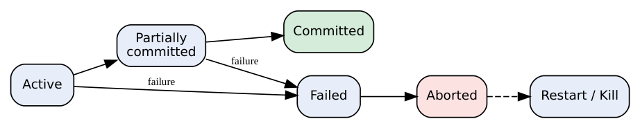
Transaction state diagram
| State | Meaning |
|---|---|
| Active | Initial state; transaction is executing |
| Partially committed | Last statement executed; changes still in memory buffer |
| Committed | Successfully completed; changes made permanent |
| Failed | Normal execution can no longer continue (error, crash) |
| Aborted | Rolled back; database restored to its state before the transaction. Then the system may restart the transaction (if failure was not a logic error) or kill it |
| (Terminated) | Either committed or aborted |
6.4 Schedules
A schedule is the chronological order in which the instructions of concurrent transactions are executed.
Serial schedule: transactions run one after another — all of T1, then all of T2. Always consistent, but no concurrency.
Concurrent (non-serial / interleaved) schedule: operations of transactions are interleaved. Better throughput and response time, but can cause problems.
Why concurrency? Advantages
Improved throughput and resource utilisation (CPU works while another transaction waits for I/O); reduced waiting/response time.
Problems of uncontrolled concurrency
| Problem | Description |
|---|---|
| Lost update | Two transactions read the same item and both update it; one update overwrites the other |
| Dirty read (temporary update / uncommitted dependency) | T2 reads a value written by T1 which later aborts → a T2 used value that “never existed” |
| Unrepeatable read | T1 reads X twice and gets different values because T2 updated X in between |
| Incorrect summary / phantom | An aggregate is computed while another transaction is updating/inserting rows |
Lost-update example:
T1 T2
read(A) A=100
 read(A) A=100
A=A−50
 A=A+20
write(A) A=50
 write(A) A=120 ← T1's update is lost (correct: 70)
6.5 Serializability
Understand it first
Running transactions one after another (serially) is always safe but slow. Running them interleaved is fast but can produce wrong results. A serializable schedule is an interleaved schedule that is guaranteed to give the same result as some one-after-another order — fast and safe. The tests below check whether a schedule has this property.
A concurrent schedule is serializable if its effect is equivalent to some serial schedule. Serializability is the accepted notion of correctness.
Conflicting instructions
Two operations conflict if they belong to different transactions, access the same data item, and at least one is a write:
| Iᵢ | Iⱼ | Conflict? |
|---|---|---|
| read(Q) | read(Q) | No |
| read(Q) | write(Q) | Yes |
| write(Q) | read(Q) | Yes |
| write(Q) | write(Q) | Yes |
Conflict serializability
Two schedules are conflict equivalent if one can be turned into the other by swapping adjacent non-conflicting operations. A schedule is conflict serializable if it is conflict equivalent to some serial schedule.
Test — precedence (serialisation) graph:
-
One node per transaction.
-
Draw an edge Tᵢ → Tⱼ if an operation of Tᵢ conflicts with and comes before an operation of Tⱼ.
-
If the graph has no cycle → conflict serializable; a topological order gives the equivalent serial schedule. If it has a cycle → not conflict serializable.
Example 1:
T1 T2
read(A)
write(A)
 read(A)
 write(A)
read(B)
write(B)
 read(B)
 write(B)
Conflicts: T1.write(A) before T2.read(A) → T1 → T2; T1.write(B) before T2.read(B) → T1 → T2. Graph: T1 → T2, no cycle ⇒ conflict serializable, equivalent to ⟨T1, T2⟩.
Example 2:
T1 T2
read(A)
 read(A)
 write(A)
write(A)
T1.read(A) before T2.write(A) → T1 → T2. T2.write(A) before T1.write(A) → T2 → T1. Cycle ⇒ not conflict serializable.
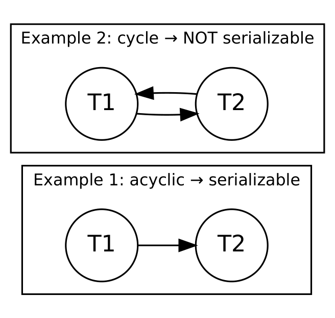
Precedence graphs for Example 1 and Example 2
View serializability
Schedules S and S’ are view equivalent if, for every data item Q:
-
Initial read: if Tᵢ reads the initial value of Q in S, it does so in S’ too.
-
Updated read (read-from): if Tᵢ reads a value of Q written by Tⱼ in S, it does so in S’ too.
-
Final write: the transaction that performs the final write of Q in S also does it in S’.
A schedule is view serializable if it is view equivalent to some serial schedule.
Every conflict-serializable schedule is view serializable, but not vice versa.
A view-serializable schedule that is not conflict serializable always contains blind writes (a write without a preceding read).
Example (view but not conflict serializable):
T1 T2 T3
read(Q)
 write(Q)
write(Q)
 write(Q)
Equivalent to serial ⟨T1, T2, T3⟩: T1 reads initial Q ✔, T3 does the final write ✔ ⇒ view serializable. Precedence graph has T1 → T2 and T2 → T1 ⇒ not conflict serializable.
| Precedence graph has T1 → T2 and | T2 → T1 ⇒ not conflict serializable. |
|---|---|
| Conflict serializability | View serializability |
| Based on swapping non-conflicting operations | Based on initial reads, read-from, final writes |
| Easy to test (precedence graph, polynomial) | Hard to test (NP-complete) |
| Stricter | More general (includes blind writes) |
| Conflict-serializable ⇒ view-serializable | View-serializable ⇏ conflict-serializable |
Recoverable and cascadeless schedules
Recoverable: if Tⱼ reads data written by Tᵢ, then Tᵢ commits before Tⱼ commits.
Cascading rollback: one transaction’s failure forces several others (that read its data) to roll back.
Cascadeless: Tⱼ reads data written by Tᵢ only after Tᵢ commits → no cascading rollbacks. Every cascadeless schedule is recoverable.
6.6 Concurrency control — Lock-based protocols

Understand it first
A lock is like the “occupied” sign on a washroom door. Many people can read a notice board at the same time (shared lock), but only one person at a time may write on it, and nobody should read while it’s being written (exclusive lock).
A lock is a variable associated with a data item that controls access to it.
| lock is a variable associated | with a data item that controls | access to it. |
|---|---|---|
| Lock | Allows | Also called |
| Shared (S) | read only; many transactions can hold S on the same item | lock-S, read lock |
| Exclusive (X) | read and write; only one transaction can hold it | lock-X, write lock |
Lock compatibility matrix:
| compatibility | matrix: | |
|---|---|---|
| S | X | |
| S | ✔ compatible | ✘ |
| X | ✘ | ✘ |
A transaction requests a lock from the lock manager; if incompatible with locks held by others, it waits.
Two-Phase Locking (2PL) protocol
Each transaction issues lock and unlock requests in two phases:
-
Growing phase: may obtain locks but may not release any.
-
Shrinking phase: may release locks but may not obtain any new lock.
The point where the transaction gets its final lock is the lock point. Ordering transactions by lock point gives an equivalent serial order ⇒ 2PL guarantees conflict serializability.
 locks held
 ▲ lock point
 │ ╱╲
 │ ╱ ╲
 │ ╱ ╲
 │ ╱ growing ╲ shrinking
 └──────────────────────────▶ time
T1: lock-X(A); read(A); A=A−50; write(A); lock-X(B); unlock(A); read(B); B=B+50; write(B);
unlock(B)
 └──────────── growing ─────────────────────┘ └────────── shrinking ──────────────┘
Problems of basic 2PL: does not prevent deadlock; may cause cascading rollback.
Variants:
Strict 2PL: hold all exclusive locks until commit/abort ⇒ cascadeless.
Rigorous 2PL: hold all locks until commit ⇒ transactions serialisable in commit order. Conservative (static) 2PL: acquire all locks before starting ⇒ deadlock-free.
Lock conversion: upgrade S → X (growing phase only), downgrade X → S (shrinking phase only).
Deadlock
A deadlock occurs when two or more transactions each wait for a lock held by another, so none can proceed (T1 holds A, wants B; T2 holds B, wants A).
Handling:
Prevention: wait-die (older waits for younger; younger requesting from older dies/rolls back) and wound-wait (older wounds — forces rollback of — younger; younger waits for older), both using timestamps; or lock everything in advance; or lock items in a fixed order. Detection & recovery: build a wait-for graph (Tᵢ → Tⱼ if Tᵢ waits for Tⱼ); a cycle = deadlock; choose a victim (least cost) and roll it back. Avoid starvation by not always choosing the same victim.
Timeout: abort a transaction that waits too long.
Starvation: a transaction waits indefinitely (e.g., repeatedly chosen as victim, or always overtaken by others) — solved by priorities/aging.
6.7 Timestamp-based protocols
Each transaction Tᵢ gets a unique timestamp TS(Tᵢ) when it starts (older = smaller). The protocol ensures the schedule is equivalent to the serial order of timestamps. For each item Q the system keeps:
W-timestamp(Q) — largest TS of any transaction that wrote Q successfully.
R-timestamp(Q) — largest TS of any transaction that read Q successfully.
Timestamp-ordering rules:
Tᵢ issues read(Q):
if TS(Tᵢ) < W-timestamp(Q) → Tᵢ needs a value already overwritten → reject, roll back Tᵢ. else execute read; R-timestamp(Q) = max(R-timestamp(Q), TS(Tᵢ)).
Tᵢ issues write(Q):
if TS(Tᵢ) < R-timestamp(Q) → a younger transaction already read Q → reject, roll back. if TS(Tᵢ) < W-timestamp(Q) → Tᵢ is writing an obsolete value → reject, roll back. else execute write; W-timestamp(Q) = TS(Tᵢ).
Rolled-back transactions restart with a new timestamp.
Thomas’ write rule: in the second write case (TS(Tᵢ) < W-timestamp(Q)) simply ignore the obsolete write instead of rolling back — allows some view-serializable schedules.
✔ Conflict serializable, deadlock-free (no waiting). ✘ Possible starvation, cascading rollbacks (unless made strict).
6.8 Multiversion concurrency control (MVCC)
Keep several versions of each data item. Each version Qₖ has its content, W-timestamp and R- timestamp.
read(Q) by Tᵢ returns the version with the largest W-timestamp ≤ TS(Tᵢ) — reads never wait and never fail.
write(Q) by Tᵢ: if TS(Tᵢ) < R-timestamp of that version → roll back Tᵢ; else create a new version (or overwrite if same timestamp). Also multiversion 2PL (read-only transactions use snapshots). Used by Oracle and PostgreSQL. ✔ High read concurrency. ✘ Extra storage; old versions need garbage collection.
6.9 Optimistic concurrency control (validation-based)
Assumes conflicts are rare: do no checking during execution; validate at the end. Each transaction runs in three phases:
-
Read (working) phase: read items and perform writes on local copies only.
-
Validation phase: check whether applying the updates would violate serializability (compare with transactions that overlapped in time).
-
Write phase: if validation succeeds, write local copies to the database; otherwise roll back and restart.
✔ No locks, no deadlock, good when conflicts are few (mostly-read workloads). ✘ Wasted work when conflicts are frequent.
6.10 Database recovery
Understand it first
The DBMS keeps a diary (the log) of every change: “T1 changed A from 1000 to 950”. After a crash, it reads the diary: changes of transactions that committed are redone (durability); changes of transactions that didn’t finish are undone (atomicity).
Failure classification
Transaction failure: logical error (bad input, overflow) or system error (deadlock).
System crash: power/OS/hardware failure — main memory lost, disk intact.
Disk (media) failure: head crash — data on disk lost (recover from backup/archive).
Storage types: volatile (RAM), non-volatile (disk), stable storage (replicated on several disks so information is never lost — used for the log).
Log-based recovery
The system keeps a log (journal) on stable storage — a sequence of records of all update activity:
<Tᵢ start>
<Tᵢ, X, V₁, V₂> — Tᵢ wrote X; old value V₁, new value V₂
<Tᵢ commit> / <Tᵢ abort>
Write-ahead logging (WAL): the log record must be written to stable storage before the corresponding data is written to the database.
Recovery operations:
undo(Tᵢ) — restore old values V₁ (scan log backwards).
redo(Tᵢ) — set new values V₂ (scan log forwards). Both are idempotent (doing them repeatedly gives the same result).
- Deferred database modification: all writes are recorded in the log but the database is updated only after the transaction commits.
Log needs only new values: <Tᵢ, X, V₂> .
After a crash: redo transactions that have both <start> and <commit> ; transactions without commit are ignored (nothing was written). No undo needed.
- Immediate database modification: database may be updated before commit (while the transaction is active).
Log needs old and new values.
After a crash: undo Tᵢ if the log has <Tᵢ start> but no <Tᵢ commit> ; redo Tᵢ if it has both.
Example log after crash:
<T0 start>
<T0, A, 1000, 950>
<T0, B, 2000, 2050>
<T0 commit>
<T1 start>
<T1, C, 700, 600>
--- crash ---
Immediate modification: redo(T0) → A = 950, B = 2050; undo(T1) → C = 700. Deferred modification: redo(T0); ignore T1 (its write never reached the DB).
Checkpoints
Problem: after a crash, searching the entire log is time-consuming and most transactions were already safely written. Checkpoint: periodically (at predetermined intervals) the system
-
writes all log records in memory to stable storage,
-
writes all modified buffer blocks to disk,
-
writes a <checkpoint L> record (L = list of active transactions).
On recovery, only transactions that were active at the last checkpoint or started after it need undo/redo; everything committed before the checkpoint is already on disk.
Shadow paging
Maintain two page tables: current page table and shadow page table (stored on disk, never modified during the transaction). Updates go to new copies of pages pointed to by the current table. Commit = atomically make the current table the new shadow table. Abort/crash = discard the current table — the shadow table still points to the old pages. ✔ No log, no undo/redo, fast recovery. ✘ Copying overhead, data fragmentation, garbage collection, hard with concurrency.
Audit trail (audit log)
A record of who accessed or changed what and when (logins, deletion of tables, privilege changes) — used for security monitoring and accountability.
6.11 Two-Phase Commit protocol (2PC) — distributed transactions
When a transaction updates data at several sites, all sites must commit or all must abort. A coordinator controls the decision.
Phase 1 — Commit-request (prepare / voting) phase — obtaining the decision
-
Coordinator writes <prepare T> to its log and sends PREPARE to all participants.
-
Each participant decides: if it can commit, it writes <ready T> to its log (forcing its updates to stable storage) and replies READY (YES); otherwise writes <no T> and replies ABORT (NO).
Phase 2 — Commit (decision) phase — performing the decision
-
If all participants replied READY → coordinator writes <commit T> and sends COMMIT to all; otherwise writes <abort T> and sends ABORT.
-
Participants commit/abort, write the result to their logs, release locks and send ACK.
-
Coordinator writes <end T> after receiving all acknowledgements.
 Coordinator Participants
 │ ── PREPARE ───────────────▶ │
 │ ◀── READY / ABORT ───────── │ Phase 1
 │ ── COMMIT / ABORT ────────▶ │
 │ ◀── ACK ─────────────────── │ Phase 2
Drawback: blocking — if the coordinator fails after participants voted READY, they must wait. (Three-phase commit addresses this.)
6.12 Security and authorisation
Security threats: unauthorised reading (loss of confidentiality), unauthorised modification (loss of integrity), denial of service (loss of availability). Security levels: database system, operating system, network, physical, human.
Authorisation = granting a user the right to access or modify data. Forms: read, insert, update, delete (on data); index, resource (create relations), alteration, drop (on schema).
Access control models
-
Discretionary Access Control (DAC) — the owner of an object decides who may access it and can pass privileges on. Implemented with SQL GRANT / REVOKE . Flexible, but a user can leak data by passing privileges.
-
Mandatory Access Control (MAC) — access determined by the system using security labels/classes (Top Secret > Secret > Confidential > Unclassified) assigned to subjects and objects. Bell–LaPadula rules: simple security property — no read up (a subject can read an object only if its clearance ≥ object’s class); star property — no write down. Users can’t override it. Used in military/government.
-
Role-Based Access Control (RBAC) — privileges are given to roles (Teacher, Student, Accountant); users are assigned roles. Easy administration.
Direct access control (as named in the syllabus) refers to discretionary control: privileges are granted directly to users by the owner.
GRANT SELECT, UPDATE ON STUDENT TO raj;
GRANT ALL ON EMP TO hr_manager WITH GRANT OPTION; -- raj can pass it on
REVOKE UPDATE ON STUDENT FROM raj; -- CASCADE/RESTRICT in standard SQL
CREATE ROLE teacher; GRANT SELECT ON RESULT TO teacher; GRANT teacher TO patel;
Role of the DBA (security) and application development
The DBA creates accounts, grants/revokes privileges, assigns security levels, monitors audit trails, takes backups and plans recovery. Database application development involves designing the schema, writing application programs (embedded/dynamic SQL, APIs like JDBC/ODBC), stored procedures, testing and tuning.
Unit 6 — Questions asked in exam
-
Define transaction. Explain the states of a transaction with a diagram.
-
Explain ACID properties with an example.
-
What is a schedule? Explain serial vs concurrent schedules; problems of concurrency.
-
Explain conflict serializability with precedence graph; view serializability; differences.
-
Write a note on the two-phase locking protocol (and its variants).
-
Explain the timestamp-ordering protocol and Thomas’ write rule.
-
Explain multiversion and optimistic (validation-based) concurrency control.
-
What is deadlock? Explain prevention and detection.
-
What is log-based recovery? Explain deferred and immediate database modification; checkpoints; shadow paging.
-
Explain the two-phase commit protocol.
-
Explain authorisation and access control (DAC, MAC, RBAC). Difference between data security and data integrity.
Unit 6 — Common mistakes
Drawing precedence edges for read–read pairs (they never conflict).
Saying 2PL prevents deadlock (basic 2PL doesn’t).
Mixing up deferred (redo only) and immediate (undo + redo) modification.
Unit 6 — Check yourself
-
Which ACID properties does the recovery manager ensure? 2. What makes a schedule not conflict serializable? 3. In 2PL, can a transaction lock a new item after releasing one?
-
In the immediate-modification log, T1 has start but no commit — undo or redo?
Answers: 1) Atomicity and durability. 2) A cycle in the precedence graph. 3) No. 4) Undo.
SQL Concepts and PL/SQL (25% of the paper)
7.1 Basics of SQL
Understand it first
SQL is the language you use to talk to a database. You say what you want (“give me names of CSE students”) and the DBMS figures out how. Four families of commands: create the structure (DDL), work with the data (DML), control permissions (DCL), control transactions (TCL).
SQL (Structured Query Language) — the standard language for relational databases (ANSI 1986, ISO). Pronounced “sequel”. Originally SEQUEL at IBM (System R).
Characteristics: declarative (say what, not how), case-insensitive keywords, statements end with ; , strings in single quotes 'CE' .
| with ; , strings | in single quotes 'CE' . |
|---|---|
| Category | Commands |
| DDL | CREATE, ALTER, DROP, TRUNCATE, RENAME |
| DML | SELECT (sometimes called DQL), INSERT, UPDATE, DELETE |
| DCL | GRANT, REVOKE |
| TCL | COMMIT, ROLLBACK, SAVEPOINT |
Common Oracle data types: NUMBER(p, s) (p digits, s after decimal), INT , CHAR(n) (fixed length), VARCHAR2(n) (variable length), DATE , TIMESTAMP , CLOB , BLOB .
7.2 DDL — creating and altering structure
CREATE TABLE DEPT (
 DeptNo NUMBER(3) PRIMARY KEY,
 Dname VARCHAR2(20) NOT NULL UNIQUE,
 Location VARCHAR2(20) DEFAULT 'Vadodara'
);
CREATE TABLE EMP (
 EmpNo NUMBER(5) CONSTRAINT pk_emp PRIMARY KEY,
 Ename VARCHAR2(30) NOT NULL,
 Job VARCHAR2(20),
 Salary NUMBER(8,2) CHECK (Salary > 0),
 HireDate DATE,
 MgrNo NUMBER(5) REFERENCES EMP(EmpNo), -- self-referencing FK
 DeptNo NUMBER(3),
 CONSTRAINT fk_dept FOREIGN KEY (DeptNo) REFERENCES DEPT(DeptNo) ON DELETE CASCADE
);
CREATE TABLE EMP_COPY AS SELECT * FROM EMP WHERE 1 = 2; -- copy structure only
ALTER TABLE
ALTER TABLE EMP ADD (Email VARCHAR2(40)); -- add column
ALTER TABLE EMP MODIFY (Ename VARCHAR2(50)); -- change type/size
ALTER TABLE EMP DROP COLUMN Email; -- remove column
ALTER TABLE EMP RENAME COLUMN Job TO Designation;
ALTER TABLE EMP ADD CONSTRAINT chk_sal CHECK (Salary <= 500000);
ALTER TABLE EMP DROP CONSTRAINT chk_sal;
Others
RENAME EMP_COPY TO EMP_BACKUP;
TRUNCATE TABLE EMP_BACKUP; -- delete all rows, keep structure, cannot roll back, fast
DROP TABLE EMP_BACKUP; -- delete structure + data
| DELETE | TRUNCATE | DROP |
|---|---|---|
| DML | DDL | DDL |
| Removes selected rows (WHERE allowed) | Removes all rows | Removes the whole table |
| Can be rolled back | Cannot be rolled back (auto- commit) | Cannot be rolled back |
| Fires triggers; slower | Faster; no row triggers | Structure, indexes, constraints gone |
Constraints (defining integrity)
| Constraint | Meaning |
|---|---|
| PRIMARY KEY | Unique + NOT NULL; one per table (can be composite: PRIMARY KEY (RollNo, CourseID) ) |
| FOREIGN KEY … REFERENCES | Value must exist in the parent table’s PK (or be NULL); ON DELETE CASCADE / ON DELETE SET NULL |
| UNIQUE | No duplicate values (NULLs allowed) |
| NOT NULL | Value required |
| CHECK (condition) | Row must satisfy the condition |
| DEFAULT value | Used when no value supplied |
Column-level constraint = written next to the column; table-level = written after all columns (needed for composite keys).
7.3 DML — INSERT, UPDATE, DELETE
INSERT INTO DEPT VALUES (10, 'Sales', 'Mumbai');
INSERT INTO DEPT (DeptNo, Dname) VALUES (20, 'HR'); -- Location gets DEFAULT
INSERT INTO EMP VALUES (1, 'Raj', 'Clerk', 25000, TO_DATE('15-06-2024','DD-MM-YYYY'), NULL,
10);
INSERT INTO EMP_BACKUP SELECT * FROM EMP WHERE DeptNo = 10; -- insert from query
INSERT INTO EMP VALUES (&EmpNo, '&Ename', ...); -- substitution variables
(SQL*Plus)
UPDATE EMP SET Salary = Salary * 1.10 WHERE Job = 'Clerk';
UPDATE EMP SET Job = 'Manager', Salary = 60000 WHERE EmpNo = 1;
DELETE FROM EMP WHERE DeptNo = 20;
DELETE FROM EMP; -- all rows
7.4 SELECT — querying
Sample data used below:
EMP
| EmpNo | Ename | Job | Salary | DeptNo | MgrNo |
|---|---|---|---|---|---|
| 1 | Amit | Manager | 60000 | 10 | NULL |
| 2 | Raj | Clerk | 25000 | 10 | 1 |
| 3 | Meet | Analyst | 45000 | 20 | 1 |
| 4 | Priya | Clerk | 28000 | 20 | 3 |
| 5 | Neha | Analyst | 50000 | 30 | 1 |
DEPT: (10, Sales, Mumbai), (20, IT, Vadodara), (30, HR, Surat), (40, Ops, Pune)
SELECT * FROM EMP; -- all columns
SELECT Ename, Salary FROM EMP; -- projection
SELECT DISTINCT Job FROM EMP; -- Manager, Clerk, Analyst
SELECT Ename, Salary*12 AS Annual_Salary FROM EMP; -- expression + alias
SELECT * FROM EMP WHERE Salary > 30000 AND DeptNo = 20; -- Meet
SELECT * FROM EMP ORDER BY Salary DESC, Ename ASC;
Operators
| Operator | Example | Meaning |
|---|---|---|
| Comparison = <> != < > <= >= | Salary <> 25000 | |
| Logical AND OR NOT | Job='Clerk' OR Job='Analyst' | |
| IN / NOT IN | DeptNo IN (10, 30) | value in a list |
| BETWEEN … AND (inclusive) | Salary BETWEEN 25000 AND 45000 | Raj, Meet, Priya |
| LIKE with % (any number of chars) and _ (exactly one) | Ename LIKE 'P%' → Priya; Ename LIKE '_e%' → Meet, Neha | pattern |
| IS NULL / IS NOT NULL | → MgrNo IS NULL Amit | (never = NULL ) |
7.5 Functions
Aggregate (group) functions — operate on many rows, return one value
| Aggregate (group) functions | — operate on many rows, | return one value |
|---|---|---|
| Function | Example | Result on EMP |
| COUNT(*) | SELECT COUNT(*) FROM EMP; | 5 (counts rows incl. NULLs) |
| COUNT(col) | COUNT(MgrNo) | 4 (ignores NULL) |
| SUM(col) | SUM(Salary) | 208000 |
| AVG(col) | AVG(Salary) | 41600 |
| MIN(col) / MAX(col) | MAX(Salary) | 60000 |
| COUNT(DISTINCT col) | COUNT(DISTINCT Job) | 3 |
GROUP BY and HAVING
SELECT DeptNo, COUNT(*) AS Emps, AVG(Salary) AS AvgSal
FROM EMP
GROUP BY DeptNo;
-- 10: 2, 42500 | 20: 2, 36500 | 30: 1, 50000
SELECT DeptNo, AVG(Salary) FROM EMP
GROUP BY DeptNo
HAVING AVG(Salary) > 40000; -- 10 (42500), 30 (50000)
Rules: every non-aggregated column in SELECT must appear in GROUP BY. WHERE filters rows before grouping; HAVING filters groups after grouping (HAVING can use aggregates, WHERE cannot).
Single-row (built-in) functions
Numeric
| Function | Example | Result |
|---|---|---|
| ABS(n) | ABS(-15) | 15 |
| CEIL(n) / FLOOR(n) | CEIL(4.2) / FLOOR(4.8) | 5 / 4 |
| ROUND(n, d) | ROUND(15.678, 2) | 15.68 |
| TRUNC(n, d) | TRUNC(15.678, 1) | 15.6 |
| MOD(m, n) | MOD(17, 5) | 2 |
| POWER(m, n) | POWER(2, 5) | 32 |
| SQRT(n) | SQRT(81) | 9 |
| SIGN(n) | SIGN(-7) | −1 |
| GREATEST/LEAST | GREATEST(4, 9, 2) | 9 |
(Oracle uses the dummy table DUAL: SELECT POWER(2,5) FROM DUAL; )
String / character
| Function | Example | Result |
|---|---|---|
| UPPER / LOWER / INITCAP | INITCAP('maher bhatt') | Maher Bhatt |
| LENGTH(s) | LENGTH('DBMS') | 4 |
| CONCAT(a, b) or a ‖ b | 'IT' ‖ 'M' | ITM |
| SUBSTR(s, start, len) | SUBSTR('DATABASE', 1, 4) | DATA |
| INSTR(s, sub) | INSTR('DATABASE', 'BASE') | 5 |
| LPAD / RPAD(s, n, c) | LPAD('7', 3, '0') | 007 |
| LTRIM / RTRIM / TRIM | TRIM(' hi ') | hi |
| REPLACE(s, a, b) | REPLACE('JACK', 'J', 'BL') | BLACK |
| TRANSLATE , REVERSE , ASCII , CHR | ASCII('A') | 65 |
Date
| Function | Example | Result |
|---|---|---|
| SYSDATE | current date/time | |
| ADD_MONTHS(d, n) | ADD_MONTHS('01-JAN-26', 3) | 01-APR-26 |
| MONTHS_BETWEEN(d1, d2) | MONTHS_BETWEEN('01-JUL- 26','01-JAN-26') | 6 |
| LAST_DAY(d) | LAST_DAY('10-FEB-26') | 28-FEB-26 |
| NEXT_DAY(d, 'day') | NEXT_DAY('09-NOV- 26','FRIDAY') | 13-NOV-26 |
| TO_CHAR(d, fmt) | TO_CHAR(SYSDATE, 'DD-MM- YYYY') | text |
| TO_DATE(s, fmt) | TO_DATE('15-08-2026','DD-MM- YYYY') | date |
| Date arithmetic | SYSDATE + 7 , d2 − d1 (days) |
Conversion/other: TO_NUMBER , NVL(expr, value) (replace NULL: NVL(MgrNo, 0) ), DECODE , CASE .
7.6 Set operations
Both queries must be union-compatible (same number of columns, compatible types).
SELECT DeptNo FROM DEPT UNION SELECT DeptNo FROM EMP; -- 10,20,30,40 (no duplicates)
SELECT DeptNo FROM DEPT UNION ALL SELECT DeptNo FROM EMP; -- keeps duplicates
SELECT DeptNo FROM DEPT INTERSECT SELECT DeptNo FROM EMP; -- 10,20,30
SELECT DeptNo FROM DEPT MINUS SELECT DeptNo FROM EMP; -- 40 (EXCEPT in standard SQL)
7.7 Joins
Understand it first
Data is split across tables (normalisation), so to answer real questions you must combine them again. A join glues rows from two tables wherever a condition matches — typically where the foreign key in one equals the primary key in the other (EMP.DeptNo =
DEPT.DeptNo).
-- INNER (equi) JOIN: matching rows only
SELECT e.Ename, d.Dname FROM EMP e JOIN DEPT d ON e.DeptNo = d.DeptNo;
SELECT e.Ename, d.Dname FROM EMP e, DEPT d WHERE e.DeptNo = d.DeptNo; -- old style
-- NATURAL JOIN: on all same-named columns
SELECT Ename, Dname FROM EMP NATURAL JOIN DEPT;
-- LEFT / RIGHT / FULL OUTER JOIN
SELECT d.Dname, e.Ename FROM DEPT d LEFT OUTER JOIN EMP e ON d.DeptNo = e.DeptNo; --
Ops appears with NULL
SELECT d.Dname, e.Ename FROM EMP e RIGHT JOIN DEPT d ON e.DeptNo = d.DeptNo; --
same result
SELECT * FROM EMP e FULL OUTER JOIN DEPT d ON e.DeptNo = d.DeptNo;
-- Oracle old syntax for outer join: WHERE e.DeptNo(+) = d.DeptNo
-- SELF JOIN: employee with manager name
SELECT e.Ename AS Employee, m.Ename AS Manager
FROM EMP e JOIN EMP m ON e.MgrNo = m.EmpNo; -- Raj-Amit, Meet-Amit, Priya-Meet,
Neha-Amit
-- CROSS JOIN: cartesian product (5 × 4 = 20 rows)
SELECT * FROM EMP CROSS JOIN DEPT;
-- NON-EQUI JOIN: condition other than '='
SELECT e.Ename, g.Grade FROM EMP e JOIN SALGRADE g ON e.Salary BETWEEN g.LoSal AND
g.HiSal;
| Join | Returns |
|---|---|
| Inner / equi | Only matching rows |
| Natural | Equi-join on same-named columns, common column shown once |
| Left outer | All left rows matches if + (NULL none) |
| Right outer | All right rows matches + |
| Full outer | All rows of both |
| Self | Table joined with itself |
| Cross | Every combination |
7.8 Sub-queries (nested queries)
Understand it first
A sub-query is a question inside a question: “Who earns more than Meet?” needs you to first find Meet’s salary (inner query), then compare everyone with it (outer query). The inner query runs first and its answer is plugged into the outer one.
A sub-query is a SELECT inside another SQL statement. The inner query runs first (for non- correlated queries) and its result is used by the outer query.
-- Single-row sub-query: employees earning more than Meet
SELECT Ename FROM EMP WHERE Salary > (SELECT Salary FROM EMP WHERE Ename = 'Meet'); --
Amit, Neha
-- Employee(s) with the highest salary
SELECT Ename FROM EMP WHERE Salary = (SELECT MAX(Salary) FROM EMP); --
Amit
-- Second highest salary
SELECT MAX(Salary) FROM EMP WHERE Salary < (SELECT MAX(Salary) FROM EMP); --
50000
-- Multi-row sub-query with IN: employees working in Vadodara
SELECT Ename FROM EMP WHERE DeptNo IN (SELECT DeptNo FROM DEPT WHERE Location =
'Vadodara'); -- Meet, Priya
-- Sub-query in FROM (inline view)
SELECT AVG(t.s) FROM (SELECT SUM(Salary) s FROM EMP GROUP BY DeptNo) t;
ANY, ALL
-- > ANY : greater than at least one value (i.e., > minimum)
SELECT Ename FROM EMP WHERE Salary > ANY (SELECT Salary FROM EMP WHERE Job = 'Clerk'); -- >
25000: Amit, Meet, Priya, Neha
-- > ALL : greater than every value (i.e., > maximum)
SELECT Ename FROM EMP WHERE Salary > ALL (SELECT Salary FROM EMP WHERE Job = 'Clerk'); -- >
28000: Amit, Meet, Neha
= ANY is the same as IN ; <> ALL is the same as NOT IN .
Correlated sub-query
The inner query refers to a column of the outer query, so it is re-executed for each row of the outer query.
-- Employees who earn more than the average of their own department
SELECT e.Ename, e.Salary, e.DeptNo
FROM EMP e
WHERE e.Salary > (SELECT AVG(x.Salary) FROM EMP x WHERE x.DeptNo = e.DeptNo);
-- Dept 10 avg 42500 → Amit; Dept 20 avg 36500 → Meet; Dept 30 avg 50000 → none
EXISTS / NOT EXISTS
EXISTS (subquery) is TRUE if the sub-query returns at least one row.
-- Departments that have at least one employee
SELECT Dname FROM DEPT d WHERE EXISTS (SELECT * FROM EMP e WHERE e.DeptNo = d.DeptNo); -
- Sales, IT, HR
-- Departments with no employee
SELECT Dname FROM DEPT d WHERE NOT EXISTS (SELECT * FROM EMP e WHERE e.DeptNo = d.DeptNo); -
- Ops
| Non-correlated sub-query | Correlated sub-query |
|---|---|
| Inner query independent of outer | Inner refers to outer’s columns |
| Executed once | Executed once per outer row |
| Faster | Slower |
7.9 Views and their types
A view is a virtual table based on the result of a SELECT. It stores only the query definition, not data (except materialised views). Querying a view runs its query on the base tables.
CREATE VIEW CUSTOMERS_VIEW AS SELECT name, age FROM CUSTOMERS;
SELECT * FROM CUSTOMERS_VIEW;
CREATE OR REPLACE VIEW EMP_DEPT_V AS
 SELECT e.Ename, d.Dname FROM EMP e JOIN DEPT d ON e.DeptNo = d.DeptNo;
CREATE VIEW CLERKS AS SELECT * FROM EMP WHERE Job = 'Clerk' WITH CHECK OPTION; --
inserts/updates must satisfy WHERE
CREATE VIEW EMP_RO AS SELECT Ename, Job FROM EMP WITH READ ONLY;
DROP VIEW EMP_RO;
Types of views
-
Simple view — based on a single table, no functions/GROUP BY/DISTINCT → usually updatable (INSERT/UPDATE/DELETE pass through to the base table).
-
Complex view — multiple tables (joins), functions, GROUP BY, DISTINCT → generally not updatable.
-
Read-only view — WITH READ ONLY .
-
Materialised view — result is physically stored and refreshed periodically (fast reporting).
-
Inline view — sub-query in the FROM clause.
Advantages: security (hide columns/rows), simplicity (hide complex joins), logical data independence, consistent customised presentation, no extra storage. Disadvantages: performance overhead for complex views, update restrictions.
7.10 Transaction control commands (TCL)
UPDATE ACCOUNT SET Bal = Bal − 500 WHERE AccNo = 1;
SAVEPOINT s1;
UPDATE ACCOUNT SET Bal = Bal + 500 WHERE AccNo = 2;
ROLLBACK TO s1; -- undo only the second update
COMMIT; -- make changes permanent and end the transaction
ROLLBACK; -- undo all changes since the last COMMIT
COMMIT — saves all changes permanently. DDL statements auto-commit.
ROLLBACK — undoes uncommitted changes.
SAVEPOINT name — marker to roll back part of a transaction.
SET TRANSACTION READ ONLY;
DCL: GRANT privilege ON object TO user [WITH GRANT OPTION]; / REVOKE privilege ON object FROM user; (see Unit 6.12).
7.11 Complex integrity constraints, assertions and triggers in SQL
Table constraints — CHECK involving several columns: CHECK (EndDate > StartDate) . Assertion — a constraint over several tables (standard SQL; rarely implemented): CREATE
ASSERTION small_club CHECK ((SELECT COUNT(*) FROM Sailors) + (SELECT COUNT(*) FROM Boats) <
100);
Triggers — procedures run automatically on events (below) — the practical way to enforce complex rules.
7.12 PL/SQL — Procedural Language extension to SQL
Understand it first
SQL can ask questions, but it can’t do “if this then that” or “repeat 100 times”. PL/SQL adds variables, IF, loops and error handling around SQL statements — making it a full
programming language that runs inside the database.
SQL alone cannot do loops, conditions or variables. PL/SQL (Oracle) adds procedural programming to SQL.
Advantages of PL/SQL (from your notes): block structure (nested, reusable, stored in DB); procedural capability (IF, loops); better performance (whole block sent to the server at once → less network traffic); error handling via exceptions; portability; security.
PL/SQL block structure
DECLARE -- optional: variables, constants, cursors
 v_name VARCHAR2(30);
 v_sal EMP.Salary%TYPE; -- same type as the column
 c_rate CONSTANT NUMBER := 0.1;
BEGIN -- mandatory: executable statements
 SELECT Ename, Salary INTO v_name, v_sal FROM EMP WHERE EmpNo = 2;
 DBMS_OUTPUT.PUT_LINE(v_name || ' earns ' || v_sal);
EXCEPTION -- optional: error handlers
 WHEN NO_DATA_FOUND THEN DBMS_OUTPUT.PUT_LINE('No such employee');
 WHEN OTHERS THEN DBMS_OUTPUT.PUT_LINE('Error: ' || SQLERRM);
END;
/
(Run SET SERVEROUTPUT ON in SQL*Plus to see output.)
Control structures
IF v_sal > 50000 THEN ... ELSIF v_sal > 30000 THEN ... ELSE ... END IF;
LOOP ... EXIT WHEN i > 10; END LOOP;
WHILE i <= 10 LOOP ... END LOOP;
FOR i IN 1..10 LOOP ... END LOOP; -- REVERSE 1..10 counts down
Predefined exceptions: NO_DATA_FOUND , TOO_MANY_ROWS , ZERO_DIVIDE , DUP_VAL_ON_INDEX , INVALID_NUMBER , OTHERS . User-defined: e EXCEPTION; … RAISE e; .
Exam programs (from your slides’ “Questions asked”)
- Sum of numbers 1 to 100
DECLARE
 s NUMBER := 0;
BEGIN
 FOR i IN 1..100 LOOP
 s := s + i;
 END LOOP;
 DBMS_OUTPUT.PUT_LINE('Sum = ' || s); -- 5050
END;
/
- Check whether a number is prime
DECLARE
 n NUMBER := &n;
 flag NUMBER := 1;
BEGIN
 IF n < 2 THEN flag := 0; END IF;
 FOR i IN 2..TRUNC(SQRT(n)) LOOP
 IF MOD(n, i) = 0 THEN flag := 0; EXIT; END IF;
 END LOOP;
 IF flag = 1 THEN DBMS_OUTPUT.PUT_LINE(n || ' is prime');
 ELSE DBMS_OUTPUT.PUT_LINE(n || ' is not prime'); END IF;
END;
/
- Insert even numbers into EVEN and odd numbers into ODD (1 to 50)
-- CREATE TABLE EVEN(num NUMBER); CREATE TABLE ODD(num NUMBER);
BEGIN
 FOR i IN 1..50 LOOP
 IF MOD(i, 2) = 0 THEN INSERT INTO EVEN VALUES (i);
 ELSE INSERT INTO ODD VALUES (i);
 END IF;
 END LOOP;
 COMMIT;
END;
/
7.13 Cursors
Understand it first
A SELECT can return many rows, but a PL/SQL variable holds one value. A cursor is like a bookmark that walks through the result rows one at a time: open the result, fetch row 1, process it, fetch row 2, … close.
A cursor is a pointer to a private memory area (context area) that holds the rows returned by a SQL statement, so PL/SQL can process them one row at a time (the “current row”).
Implicit cursor
Created automatically by Oracle for every DML statement (INSERT/UPDATE/DELETE) and single-row SELECT INTO. Named SQL . Attributes:
| Attribute | Meaning |
|---|---|
| SQL%FOUND | TRUE if the statement affected ≥ 1 row |
| SQL%NOTFOUND | TRUE if no row affected |
| SQL%ROWCOUNT | Number of rows affected |
| SQL%ISOPEN | Always FALSE for implicit cursors (auto-closed) |
BEGIN
 UPDATE EMP SET Salary = Salary * 1.05 WHERE DeptNo = 20;
 IF SQL%FOUND THEN DBMS_OUTPUT.PUT_LINE(SQL%ROWCOUNT || ' rows updated'); END IF;
END;
/
Explicit cursor
User-defined for a SELECT that returns more than one row. Steps: DECLARE → OPEN → FETCH → CLOSE (SQL Server also DEALLOCATE). Attributes: cur%FOUND , cur%NOTFOUND , cur%ROWCOUNT , cur%ISOPEN .
DECLARE
 CURSOR c_emp IS SELECT Ename, Salary FROM EMP WHERE DeptNo = 10;
 v_name EMP.Ename%TYPE;
 v_sal EMP.Salary%TYPE;
BEGIN
 OPEN c_emp;
 LOOP
 FETCH c_emp INTO v_name, v_sal;
 EXIT WHEN c_emp%NOTFOUND;
 DBMS_OUTPUT.PUT_LINE(v_name || ' ' || v_sal);
 END LOOP;
 CLOSE c_emp;
END;
/
Cursor FOR loop (opens, fetches, closes automatically):
BEGIN
 FOR r IN (SELECT Ename, Salary FROM EMP) LOOP
 DBMS_OUTPUT.PUT_LINE(r.Ename || ' ' || r.Salary);
 END LOOP;
END;
/
Slides’ example (SQL Server syntax) — copy CE students into STUDENT1:
DECLARE @rno INT, @name VARCHAR(50), @branch VARCHAR(50);
DECLARE cursor_student CURSOR FOR SELECT rno, name, branch FROM student;
OPEN cursor_student;
FETCH NEXT FROM cursor_student INTO @rno, @name, @branch;
WHILE @@FETCH_STATUS = 0
BEGIN
 IF (@branch = 'CE') INSERT INTO student1 VALUES (@rno, @name, @branch);
 FETCH NEXT FROM cursor_student INTO @rno, @name, @branch;
END;
CLOSE cursor_student;
DEALLOCATE cursor_student;
Exam Q7 — explicit cursor: top 5 customers by fixed-deposit amount Tables:
cust_mstr(custno, name, occupation), fd_dtls(fd_ser_no, fd_no, type, period, opndt, duedt, amt, dueamt), acct_fd_cust_dtls(acct_fd_no, custno).
DECLARE
 CURSOR c_fd IS
 SELECT c.name, f.fd_no, f.amt
 FROM cust_mstr c, acct_fd_cust_dtls a, fd_dtls f
 WHERE c.custno = a.custno AND a.acct_fd_no = f.fd_no
 ORDER BY f.amt DESC;
 v_name cust_mstr.name%TYPE;
 v_fdno fd_dtls.fd_no%TYPE;
 v_amt fd_dtls.amt%TYPE;
BEGIN
 OPEN c_fd;
 LOOP
 FETCH c_fd INTO v_name, v_fdno, v_amt;
 EXIT WHEN c_fd%NOTFOUND OR c_fd%ROWCOUNT > 5;
 DBMS_OUTPUT.PUT_LINE(v_name || ' ' || v_fdno || ' ' || v_amt);
 END LOOP;
 CLOSE c_fd;
END;
/
7.14 Stored procedures
A stored procedure is a named group of PL/SQL statements stored (pre-compiled) in the database that performs a specific task. It has a header (name + parameters) and a body (declaration, execution, exception sections). It may return zero, one or several values through OUT parameters.
Parameter modes: IN (send a value in — default), OUT (get a value back), IN OUT (both).
CREATE OR REPLACE PROCEDURE raise_salary (p_empno IN NUMBER, p_pct IN NUMBER, p_newsal OUT
NUMBER)
AS
BEGIN
 UPDATE EMP SET Salary = Salary * (1 + p_pct/100) WHERE EmpNo = p_empno;
 SELECT Salary INTO p_newsal FROM EMP WHERE EmpNo = p_empno;
 COMMIT;
EXCEPTION
 WHEN NO_DATA_FOUND THEN DBMS_OUTPUT.PUT_LINE('Employee not found');
END;
/
-- Execute
EXEC raise_salary(2, 10, :x); -- from SQL*Plus (x is a bind variable)
DECLARE s NUMBER; BEGIN raise_salary(2, 10, s); DBMS_OUTPUT.PUT_LINE(s); END; -- from
another block
DROP PROCEDURE raise_salary;
SQL Server form (as in your slides):
CREATE PROCEDURE get_studentname_by_id @id INT
AS
SELECT studentname FROM student WHERE studentID = @id;
EXEC get_studentname_by_id 10;
Advantages: security (grant EXECUTE only), faster (pre-compiled), code sharing/reuse, productivity, less network traffic, central maintenance.
7.15 Stored functions
Like a procedure but must return exactly one value with RETURN , and can be used inside SQL expressions.
CREATE OR REPLACE FUNCTION annual_sal (p_empno NUMBER) RETURN NUMBER
AS
 v_sal NUMBER;
BEGIN
 SELECT Salary * 12 INTO v_sal FROM EMP WHERE EmpNo = p_empno;
 RETURN v_sal;
END;
/
SELECT Ename, annual_sal(EmpNo) FROM EMP;
| Procedure | Function |
|---|---|
| May return 0, 1 or many values (OUT params) | Must return exactly one value (RETURN) |
| Called as a statement: EXEC proc; | Called in an expression / SELECT |
| Used for actions (DML) | Used for computations |
Exam Q8 — f_ChkAcctNo and a deposit/withdrawal block
-- ACCOUNT(acct_no, name, type, balance)
CREATE OR REPLACE FUNCTION f_ChkAcctNo (p_acct VARCHAR2) RETURN NUMBER
AS
 cnt NUMBER;
BEGIN
 SELECT COUNT(*) INTO cnt FROM ACCOUNT WHERE acct_no = p_acct;
 IF cnt > 0 THEN RETURN 1; ELSE RETURN 0; END IF;
END;
/
DECLARE
 v_acct ACCOUNT.acct_no%TYPE := '&acct_no';
 v_type CHAR(1) := '&D_or_W'; -- D = deposit, W = withdrawal
 v_amt NUMBER := &amount;
BEGIN
 IF f_ChkAcctNo(v_acct) = 1 THEN
 IF v_type = 'D' THEN
 UPDATE ACCOUNT SET balance = balance + v_amt WHERE acct_no = v_acct;
 ELSE
 UPDATE ACCOUNT SET balance = balance - v_amt WHERE acct_no = v_acct;
 END IF;
 COMMIT;
 DBMS_OUTPUT.PUT_LINE('Transaction successful');
 ELSE
 DBMS_OUTPUT.PUT_LINE('Account ' || v_acct || ' does not exist');
 END IF;
END;
/
7.16 Database triggers
Understand it first
A trigger is an automatic reaction: “whenever someone updates a salary, automatically write the old and new salary into an audit table.” Nobody calls it — the event fires it, like a motion-sensor light.
A trigger is a stored PL/SQL block that executes automatically when a specified event occurs on a table/view (INSERT, UPDATE, DELETE), or on DDL/logon events.
When/why to use triggers (need & advantages): update another table when one table changes; maintain derived columns automatically; auditing/logging; enforce complex business rules and integrity beyond CHECK; prevent invalid transactions; replicate data.
Types
By timing: BEFORE, AFTER, INSTEAD OF (for views).
By level: row-level ( FOR EACH ROW — fires once per affected row; can use :NEW and :OLD ) and statement-level (fires once per statement).
By event: DML triggers, DDL triggers (CREATE/ALTER/DROP), logon/system triggers (SQL Server/Oracle).
Oracle syntax
CREATE [OR REPLACE] TRIGGER trigger_name
{BEFORE | AFTER | INSTEAD OF} {INSERT [OR] | UPDATE [OF col] [OR] | DELETE}
ON table_name
[FOR EACH ROW]
[WHEN (condition)]
DECLARE ... BEGIN ... EXCEPTION ... END;
-- Audit every salary change
CREATE OR REPLACE TRIGGER trg_sal_audit
AFTER UPDATE OF Salary ON EMP
FOR EACH ROW
BEGIN
 INSERT INTO SAL_AUDIT VALUES (:OLD.EmpNo, :OLD.Salary, :NEW.Salary, SYSDATE);
END;
/
-- Business rule: salary may not decrease
CREATE OR REPLACE TRIGGER trg_no_cut
BEFORE UPDATE OF Salary ON EMP
FOR EACH ROW
WHEN (NEW.Salary < OLD.Salary)
BEGIN
 RAISE_APPLICATION_ERROR(-20001, 'Salary cannot be reduced');
END;
/
SQL Server form (as in your slides):
CREATE TRIGGER student_msg ON Student
AFTER INSERT, UPDATE, DELETE
AS
BEGIN
 PRINT 'One record is affected'
END;
-- SQL Server DML triggers: AFTER (FOR) triggers run after the statement succeeds;
-- INSTEAD OF triggers run in place of the statement (the original DML does not happen).
| Trigger | Stored procedure |
|---|---|
| Fires automatically on an event | Called explicitly |
| No parameters | Can take parameters |
| Cannot return values | Can return values (OUT) |
| Cannot use COMMIT/ROLLBACK (Oracle) | Can |
7.17 SQL query practice set (write these until fluent)
| Schema: STUDENT(RollNo, Name, | Branch, Sem, SPI, City) | |
|---|---|---|
| # | Query | SQL |
| 1 | Students of CE with SPI > 8 | SELECT * FROM STUDENT WHERE Branch='CE' AND SPI>8; |
| 2 | Names starting with ‘M’ | SELECT Name FROM STUDENT WHERE Name LIKE 'M%'; |
| 3 | Count students per branch | SELECT Branch, COUNT(*) FROM STUDENT GROUP BY Branch; |
| 4 | Branches having more than 30 students | … GROUP BY Branch HAVING COUNT(*) > 30; |
| 5 | Topper’s name | SELECT Name FROM STUDENT WHERE SPI = (SELECT MAX(SPI) FROM STUDENT); |
| 6 | Students from Vadodara or Surat | … WHERE City IN ('Vadodara','Surat'); |
| 7 | Average SPI of Sem 3, rounded to 2 | SELECT ROUND(AVG(SPI),2) FROM STUDENT WHERE Sem=3; |
| 8 | Increase SPI by 0.5 for EE | UPDATE STUDENT SET SPI = SPI + 0.5 WHERE Branch='EE'; |
| 9 | Delete students with SPI < 4 | DELETE FROM STUDENT WHERE SPI < 4; |
| 10 | Students not enrolled in any course | SELECT Name FROM STUDENT s WHERE NOT EXISTS (SELECT * FROM ENROLL e WHERE e.RollNo=s.RollNo); |
| 11 | Names in uppercase with length | SELECT UPPER(Name), LENGTH(Name) FROM STUDENT; |
| 12 | Add Email column | ALTER TABLE STUDENT ADD Email VARCHAR2(40); |
Unit 7 — Questions asked in exam
-
Explain DDL, DML, DCL, TCL commands with examples. Difference between DELETE, TRUNCATE, DROP.
-
Explain constraints (PK, FK, UNIQUE, NOT NULL, CHECK) with syntax.
-
Explain aggregate, numeric, string and date functions with examples.
-
Write SQL queries for a given schema (joins, GROUP BY/HAVING, sub-queries, correlated, EXISTS, ANY/ALL, set operations).
-
What is a view? Types; advantages.
-
Write PL/SQL blocks: sum 1–100; prime check; even/odd tables.
-
Explain cursors (implicit, explicit) with example; cursor attributes.
-
Explain stored procedures with example; procedure vs function.
-
What are triggers? Types, need/advantages, example.
Unit 7 — Common mistakes
Using WHERE with an aggregate ( WHERE AVG(Sal) > … ) — must be HAVING.
Writing = NULL instead of IS NULL .
Selecting a non-aggregated column that isn’t in GROUP BY.
Forgetting EXIT WHEN cur%NOTFOUND in a cursor loop (infinite loop).
Unit 7 — Check yourself
- Delete all rows but keep the table, fastest way? 2. Query: departments with average salary above 40000. 3. Difference between procedure and function? 4. Which cursor attribute gives the number of rows affected?
Answers: 1) TRUNCATE. 2) SELECT DeptNo FROM EMP GROUP BY DeptNo HAVING AVG(Salary) > 40000; 3) Function must return one value and can be used in SQL; procedure returns via OUT
parameters and is called as a statement. 4) %ROWCOUNT.
Last-Night Revision Sheet (DBMS)
U1 DBMS = software to manage related data efficiently + securely. File-system problems = redundancy, inconsistency, isolation, integrity, atomicity, concurrency, security. 3 levels: internal (how stored) / conceptual (what) / external (views). Physical independence = change storage without changing logical schema; logical independence = change logical schema without changing views (harder). Query processor (DDL interpreter, DML compiler, evaluation engine) + storage manager (authorization, transaction, file, buffer managers).
U2 Rectangle entity, ellipse attribute, diamond relationship, double rectangle weak entity, double diamond identifying relationship, double ellipse multivalued, dashed ellipse derived, double line total participation. Cardinality 1:1, 1:N, M:N. Weak entity PK = owner PK + discriminator. Specialisation (top-down) / generalisation (bottom-up); constraints: disjoint/overlapping, total/partial, condition/user-defined. Aggregation = relationship treated as entity. M:N → separate table. Integrity: domain, entity (PK not null), referential (FK matches or NULL).
U3 σ rows, π columns, × all pairs (n₁n₂ rows, d₁+d₂ cols), ∪ ∩ − need union compatibility, ⋈ natural join, ÷ “for all”, ρ rename, 𝒢 aggregate. TRC {t | P(t)}, DRC {⟨x…⟩ | P}. SQL order: FROM → WHERE → GROUP BY → HAVING → SELECT → ORDER BY.
U4 X → Y. Armstrong: reflexivity, augmentation, transitivity (+ union, decomposition, pseudo- transitivity). X⁺ algorithm → super key if X⁺ = R. Canonical cover: split RHS, remove extraneous LHS attrs, remove redundant FDs. Lossless if R₁∩R₂ → R₁ or R₂. 1NF atomic; 2NF no partial; 3NF no transitive (X super key or A prime); BCNF every determinant super key; 4NF no MVD; 5NF no join dependency.
U5 Parse/translate → optimise → evaluate. Cost = block transfers + seeks. A1 linear b_r, A2 binary ⌈log₂ b_r⌉. Joins: nested n_R·b_S + b_R; block nested b_R·b_S + b_R; merge b_R + b_S; hash 3(b_R + b_S); smaller relation outside. Materialisation (temp tables) vs pipelining (pass tuples). Heuristic: push σ and π down.
U6 ACID (atomicity & durability → recovery; isolation → concurrency control). States: active → partially committed → committed; failed → aborted. Conflict = different txns, same item, ≥1 write. Precedence graph acyclic ⇒ conflict serializable. View serializable: initial read, read-from, final write. 2PL: growing then shrinking; strict 2PL holds X locks till commit. Timestamp: reject if TS(T) < W-ts (read) or < R-ts/W-ts (write); Thomas rule ignores obsolete writes. MVCC: reads never wait. Optimistic: read → validate → write. Deferred modification: redo only; immediate: undo + redo. Checkpoint shortens recovery. 2PC: prepare/vote, then commit/abort. DAC (GRANT/REVOKE), MAC (labels, no read up/no write down), RBAC (roles).
U7 DDL/DML/DCL/TCL. Constraints PK, FK, UNIQUE, NOT NULL, CHECK, DEFAULT. WHERE vs HAVING. Joins inner/outer/self/cross. ANY = vs at least one, ALL = vs every. Correlated sub- query runs per outer row. EXISTS tests non-empty. View = virtual table (simple updatable / complex). PL/SQL block DECLARE-BEGIN-EXCEPTION-END. Cursor: implicit
(SQL%ROWCOUNT) / explicit (DECLARE-OPEN-FETCH-CLOSE). Procedure (IN/OUT/IN OUT) vs function (RETURN). Trigger: BEFORE/AFTER/INSTEAD OF, row/statement, :NEW/:OLD.