Last-Night Revision Sheet (DSA)
Read This First
What this subject is about, in plain words
A computer program does two things: it stores data and it does something with that data.
Data structure = how you arrange data in memory.
Algorithm = the step-by-step method you use to work on that data.
Example from real life. You have 500 phone numbers. - Written on random scraps of paper in a box → to find “Raj” you check every scrap (slow). - Written in a notebook sorted A–Z → open in the middle, decide left or right half, repeat (fast). Same data, different arrangement (data structure), and therefore a different, faster method (algorithm). That’s the entire subject in one example.
Every chapter in this subject introduces one way of arranging data — array, stack, queue, linked list, tree, graph, hash table — and the operations you can do on it (insert, delete, search, traverse), along with how fast those operations are.
How each topic is taught in this guide
In one line — the whole idea in a sentence.
Understand it — plain words + a real-life comparison + a picture.
How it works, step by step — with a traced example where every step is shown.
Code, explained line by line (in C, the language of your lab).
Common mistakes and what to write in the exam.
Check yourself — quick questions with answers.
C refresher — just what you need
You’ll see these in the code. Read once; come back whenever confused.
| code | Meaning |
|---|---|
| int a[5]; | an array of 5 integers: a[0] … a[4] |
| struct node { int data; struct node *next; }; | a custom type holding an int and a pointer |
| int *p; | p is a pointer — a variable that holds a memory address |
| p = &x; | p now holds the address of x (“&” = “address of”) |
| *p | the value stored at the address in p (“go to that address”) |
| p->data | for a pointer to a struct: “the data field of the struct points to” (same as (*p).data ) |
| NULL | a special pointer value meaning “points to nothing” |
| malloc(sizeof(struct node)) | ask the system for memory for one node; returns its address |
| free(p) | give that memory back |
Pointer analogy: a variable is a house holding a value. A pointer is a piece of paper with the house’s address written on it. *p means “go to the address on the paper and look inside the house”.
Syllabus and marks
| Unit | Topic | Weightage |
|---|---|---|
| 1 | Introduction: pseudocode, ADT, data types, linear/non-linear, asymptotic notation | 10 |
| 2 | Recursion: factorial, Tower of Hanoi, Fibonacci | 5 |
| 3 | Linear lists: array, stack, Polish notation, queue (circular, priority, deque), linked lists | 20 |
| 4 | Trees: binary tree, traversals, threaded tree, BST, general → binary | 20 |
| 5 | Graphs: terminology, matrix/list representation, DFS, BFS | 20 |
| 6 | Searching & sorting: selection, insertion, bubble, quick, external sort, linear/binary search, hashing | 15 |
Your CET pattern: 1-mark MCQs, 3-mark “define/differentiate”, 5-mark “explain + algorithm”, 7- mark “full algorithm + trace with an example”. So for every topic you need: definition, diagram, algorithm, a traced example, and the time complexity.
How to write an algorithm in your professor’s style (Tremblay & Sorenson):
Procedure PUSH(S, TOP, X)
1. [Check for stack overflow]
 If TOP ≥ N − 1 then Write('STACK OVERFLOW'); Return
2. [Increment TOP]
 TOP ← TOP + 1
3. [Insert element]
 S[TOP] ← X
4. [Finished]
 Return
Numbered steps, a short comment in [square brackets] saying what each step does, and ← for “gets the value”.
Introduction: Data Structures, ADTs and Algorithm Efficiency
1.1 Data, information, data structure, algorithm
Data = raw facts with no meaning on their own: 72.5, 71.8, 73.1 or ["Alice", "Bob"] . Information = data after processing, which now means something: “the average temperature was 72.5°F”.
Basic terminology (from your Unit-1 notes)
Imagine a college office keeping student records:
| a college office keeping | student records: | |
|---|---|---|
| Term | Meaning | In the student-records example |
| Data item | a single unit of value | a roll number |
| Group item | a data item made of sub-items | Name → first, middle, last |
| Elementary item | cannot be divided further | age |
| Entity | a thing that has attributes | one student |
| Attribute / field | a property of an entity | name, branch, SPI |
| Entity set | all entities of the same type | all students |
| Record | all field values of one entity | (25C21007, Maher, CSE, 8.5) |
| File | a collection of records | the whole student file |
| Key / primary key | a field that uniquely identifies a record | enrolment number |
Data structure
Definition: a data structure is a way of organising and storing data in memory so that it can be used efficiently. It specifies (1) how data is laid out, (2) how items are related, and (3) which operations can be done on it.
Algorithm
Definition: an algorithm is a finite set of clear, step-by-step instructions that solves a problem.
Library analogy (from your notes): books = data; shelves arranged by subject and author = data structure; the librarian’s method of finding a book = algorithm. Without the shelves, even the smartest librarian is slow.
Program = Algorithm + Data Structure (Niklaus Wirth).
Properties (characteristics) of an algorithm — memorise all six
| Properties (characteristics) | of an algorithm — memorise | all six |
|---|---|---|
| Property | Meaning | What goes wrong without it |
| Input | zero or more inputs | — |
| Output | at least one output | an algorithm that produces nothing is useless |
| Definiteness | every step is clear and unambiguous | “add a few numbers” — how many? |
| Finiteness | it must stop after a finite number of steps | an infinite loop never gives an answer |
| Effectiveness | every step is simple enough to actually carry out | “find the largest prime” — impossible |
| Correctness | gives the right answer for every valid input |
Why do we need data structures?
Speed: the right structure makes search/insert/delete fast (binary search on a sorted array takes 20 steps for a million items; checking one by one takes up to a million).
Memory efficiency: store only what’s needed.
Reusability: a stack written once can be used in many programs.
Abstraction: users use the operations without knowing the details.
1.2 Pseudocode
In one line: an algorithm written in structured English, looking like code but ignoring the exact rules (syntax) of any programming language.
It’s for humans — to plan and explain an algorithm before coding. A compiler can’t run it.
Common conventions:
One instruction per line, indent the inside of loops/ifs.
← for assignment, = for comparison.
IF … THEN … ELSE … ENDIF , WHILE … DO … ENDWHILE , FOR i ← 1 TO n DO … ENDFOR , READ , WRITE , RETURN .
Example — largest of n numbers:
Algorithm MAX(A, n)
1. max ← A[1] // assume the first is largest
2. FOR i ← 2 TO n DO // look at every other number
3. IF A[i] > max THEN max ← A[i] // found a bigger one? remember it
4. ENDFOR
5. RETURN max
Trace with A = [4, 9, 2, 7]: max = 4 → 9 > 4 so max = 9 → 2 no → 7 no → return 9.
Advantages: language-independent, easy to understand and to convert into any language, easy to spot logic errors. Disadvantages: no standard form, can’t be executed or tested directly.
1.3 Data types — primitive and non-primitive
A data type tells the computer what kind of value a variable holds and what operations are allowed (you can multiply ints, you can’t multiply names).
Classification of data structures (draw this in every “classify” question)
 DATA STRUCTURES
 ┌─────────────┴──────────────┐
 PRIMITIVE NON-PRIMITIVE
 int, float, char, ┌──────────┴──────────┐
 double, boolean, LINEAR NON-LINEAR
 pointer ┌──────┼──────┐ ┌────┴────┐
 Array Stack Queue Tree Graph
 Linked list
Primitive data structures — the basic types built into the language and directly handled by the machine. Each holds one value. int , float , char , double , boolean , pointer . Non-primitive data structures — built by the programmer out of primitive types; they hold collections of values with relationships. Arrays, stacks, queues, lists, trees, graphs, files.
Analogy: primitive types are single LEGO bricks; non-primitive structures are things you build from many bricks.
| Primitive | Non-primitive |
|---|---|
| Holds a single value | Holds a group of values |
| Built into the language | Made by the programmer |
| Operated on directly by machine instructions | Operated on by algorithms |
| int, char, float | array, stack, tree |
Linear vs non-linear
Linear: elements are arranged in a sequence, one after another — each element has exactly one before it and one after it (except the ends). You can visit all of them in one straight pass. → array, stack, queue, linked list.
Non-linear: elements are arranged in a hierarchy (tree) or a network (graph) — one element can be connected to many others. You can’t visit them all in one straight line. → tree, graph.
Linear: [A] → [B] → [C] → [D] (a train of coaches)
 Non-linear: A (a family tree)
 / \
 B C
 / \
 D E
| Linear | Non-linear |
|---|---|
| Single level | Multiple levels |
| All elements visited in one run | Needs special traversals (in-order, DFS, BFS) |
| Easy to implement | Harder to implement |
| Can waste memory (arrays) | Uses memory efficiently |
| Array, stack, queue, linked list | Tree, graph |
Other ways to classify
Static vs dynamic: static = fixed size decided before running (array of 100). Dynamic = grows and shrinks while running (linked list).
Homogeneous vs heterogeneous: homogeneous = all elements of the same type (int array). Heterogeneous = mixed types (a struct with name + age + marks).
Contiguous vs linked: array elements sit side by side in memory; linked-list nodes are scattered and joined by pointers.
Operations on data structures
| Operation | Meaning |
|---|---|
| Traversing | visiting each element exactly once (e.g., to print all) |
| Searching | finding where an element is |
| Inserting | adding a new element |
| Deleting | removing an element |
| Sorting | arranging in order |
| Merging | combining two sorted structures into one sorted one |
1.4 Abstract Data Type (ADT)
In one line: an ADT describes what a data type does (its values and operations), not how it’s done inside.
Understand it
TV remote analogy: you know the buttons — power, volume up, channel 5 — and what each does. You have no idea about the circuit inside, and you don’t need to. The list of buttons and what they do is the ADT. The circuit is the implementation (the data structure). If the company changes the circuit but keeps the same
buttons, you can still use the remote exactly the same way.
So:
ADT = the “what” — a list of operations and rules, like a contract.
Data structure = the “how” — the actual arrangement in memory (array or linked list) and code.
Components of an ADT
-
Data/values it can hold.
-
Operations allowed on them.
-
Rules (axioms) the operations must obey (pre- and post-conditions).
-
Error conditions (e.g., removing from an empty stack).
The ADT model
 ┌────────────────────────────────────────┐
 Application │ PUBLIC INTERFACE (what users see) │
 program ──▶│ push(), pop(), peek(), isEmpty() │
 ├────────────────────────────────────────┤
 │ PRIVATE IMPLEMENTATION (hidden) │
 │ data structure: array or linked list │
 │ + the code of each function │
 └────────────────────────────────────────┘
The program can reach the data only through the interface functions. This hiding of details is called encapsulation (or information hiding).
Example: the Stack ADT
ADT Stack
 Values: an ordered collection; insertions and deletions only at one end (top)
 Operations:
 create() → an empty stack
 push(S, x) → puts x on top
 pop(S) → removes and returns the top item (error if empty)
 peek(S) → returns the top item without removing (error if empty)
 isEmpty(S) → true if no items
 isFull(S) → true if no space (array version)
 Rules:
 after push(S, x), pop(S) returns x
 isEmpty(create()) = true
ADT implementation
The same ADT can be built in different ways — the user doesn’t notice:
| same ADT can be built | in different ways — the user doesn’t | notice: |
|---|---|---|
| ADT | Implementation 1 | Implementation 2 |
| Stack | array | linked list |
| Queue | array circular | linked list |
| List | array | linked list |
| Priority queue | array | heap |
In C, the interface goes in a header file ( stack.h — function prototypes) and the implementation in stack.c .
Advantages of ADTs: encapsulation; you can change the implementation without changing user programs (modularity); reusability; easier to prove correct.
1.5 Algorithm efficiency — time and space complexity
Why analyse algorithms?
Two programs can solve the same problem, but one might take 1 second and the other 3 hours on big data. We need a way to compare algorithms without running them and independent of the computer, language or programmer.
Time complexity = how the number of basic steps grows as the input size n grows. Space complexity = how the extra memory needed grows with n. (Fixed part: code, simple variables. Variable part: arrays created, recursion stack.)
Counting steps — the frequency count method
sum = 0; // runs 1 time
for (i = 0; i < n; i++) // condition checked n+1 times
 sum = sum + a[i]; // runs n times
return sum; // 1 time
Total ≈ 1 + (n + 1) + n + 1 = 2n + 3. For big n, the “2” and “+3” hardly matter; what matters is that the time grows in proportion to n → O(n).
Best, worst and average case
Searching for a number in a list of n numbers, checking one by one:
Best case: it’s the first element → 1 comparison.
Worst case: it’s the last element, or not there → n comparisons.
Average case: on average about n/2.
The worst case is the most important: it’s a guarantee (“it will never take longer than this”).
Loop patterns — how to find complexity quickly (your Algorithm Analysis notes)
| Loop patterns — how to find | complexity quickly (your Algorithm | Analysis |
|---|---|---|
| Code | How many times the body runs | Complexity |
| for(i=0; i<n; i++) | n | O(n) |
| for(i=0; i<n; i+=2) | n/2 (constants don’t matter) | O(n) |
| for(i=1; i<n; i*=2) | i = 1, 2, 4, 8 … until n → log₂n times | O(log n) |
| for(i=n; i>1; i/=2) | n, n/2, n/4 … 1 → log₂n | O(log n) |
| two loops nested, each to n | n × n | O(n²) |
| for(i=0;i<n;i++) for(j=0;j<i;j++) | 0 + 1 + … + (n−1) = n(n−1)/2 | O(n²) |
| outer to n, inner j*=2 | n × log n | O(n log n) |
| for(i=1; i*i<=n; i++) | √n | O(√n) |
| two loops one after another | n + n = 2n | O(n) |
Three rules: loops one after another → add; loops inside each other → multiply; keep only the biggest term and drop constants.
Why does i *= 2 give log n? i takes values 1, 2, 4, 8, …, 2ᵏ. The loop stops when 2ᵏ ≥ n, i.e., k = log₂n. For n = 1,000,000 that’s only ~20 iterations!
1.6 Asymptotic notations — O, Ω, Θ
“Asymptotic” = what happens as n becomes very large. We describe the growth rate of the running time f(n) by comparing it with a simple function g(n) like n, n², log n.
Big-O — upper bound (“at most”)
Definition: f(n) = O(g(n)) if there exist positive constants c and n₀ such that
0 ≤𝑓( 𝑛) ≤𝑐⋅𝑔( 𝑛)
for all 𝑛≥𝑛0
Meaning: after some point n₀, f(n) never grows faster than c·g(n). It’s a ceiling → used for the worst case.
Worked example: f(n) = 3n + 2. Show f(n) = O(n). We need c and n₀ with 3n + 2 ≤ c·n. Try c = 4: 3n + 2 ≤ 4n ⇔ 2 ≤ n. So it holds for all n ≥ 2. c = 4, n₀ = 2 ✔.
Big-Omega (Ω) — lower bound (“at least”)
Definition: f(n) = Ω(g(n)) if there exist positive c, n₀ such that
0 ≤𝑐⋅𝑔( 𝑛) ≤𝑓( 𝑛)
for all 𝑛≥𝑛0
Meaning: f(n) grows at least as fast as g(n). A floor → best case. Example: 3n + 2 ≥ 3n for all n ≥ 1 → 3n + 2 = Ω(n) with c = 3, n₀ = 1.
Big-Theta (Θ) — tight bound (“exactly this order”)
Definition: f(n) = Θ(g(n)) if there exist positive c₁, c₂, n₀ such that
0 ≤𝑐1𝑔( 𝑛) ≤𝑓( 𝑛) ≤𝑐2𝑔( 𝑛)
for all 𝑛≥𝑛0
Meaning: f(n) is sandwiched between two multiples of g(n) — it grows exactly like g(n). Example: 3n ≤ 3n + 2 ≤ 4n for n ≥ 2 → 3n + 2 = Θ(n) with c₁ = 3, c₂ = 4, n₀ = 2. Example 2: f(n) = 2n² + 3n + 1. Lower: 2n² ≤ f(n). Upper: 2n² + 3n + 1 ≤ 2n² + 3n² + n² = 6n² for n ≥ 1. So Θ(n²), c₁ = 2, c₂ = 6, n₀ = 1.
 time ▲ c₂·g(n)
 │ ╱
 │ ╱ ← f(n) stays between the two lines after n₀
 │ ╱ ╱
 │ ╱ ╱ ── c₁·g(n)
 │ ╱ ╱ ──
 │ ╱╱──
 └───┼──────────────────▶ n
 n₀
| Notation | Bound | Like | Used for |
|---|---|---|---|
| O | upper | ≤ | worst case |
| Ω | lower | ≥ | best case |
| Θ | tight | = | exact growth |
(Little-o and little-ω are the strict versions, < and >.)
Growth rates — memorise this order
| 1 < | log 𝑛< √𝑛< 𝑛< | 𝑛log 𝑛< | 𝑛2 < 𝑛3 < 2𝑛< 𝑛! < 𝑛𝑛 | |
|---|---|---|---|---|
| n | log₂n | n log n | n² | 2ⁿ |
| 8 | 3 | 24 | 64 | 256 |
| 16 | 4 | 64 | 256 | 65,536 |
| 1024 | 10 | 10,240 | ≈ 10⁶ | a number with 309 digits |
Names: O(1) constant, O(log n) logarithmic, O(n) linear, O(n log n) linearithmic, O(n²) quadratic, O(n³) cubic, O(2ⁿ) exponential, O(n!) factorial.
Properties of asymptotic notations
-
Reflexive: f(n) = O(f(n)) (also Ω, Θ).
-
Transitive: f = O(g) and g = O(h) ⇒ f = O(h).
-
Symmetric (only Θ): f = Θ(g) ⇔ g = Θ(f).
-
Transpose symmetry: f = O(g) ⇔ g = Ω(f).
-
Constants don’t matter: if f = O(g), then 7·f = O(g).
-
Sum rule: f₁ + f₂ = O(max(g₁, g₂)) — e.g., n² + n = O(n²).
-
Product rule: f₁ · f₂ = O(g₁ · g₂) — e.g., a loop of n containing an O(log n) step = O(n log n).
-
Polynomials: a polynomial of degree d is Θ(nᵈ): 5n³ + 2n² + 7 = Θ(n³).
-
If f = O(g) and f = Ω(g), then f = Θ(g).
Complexities to remember
| Operation / algorithm | Best | Average | Worst |
|---|---|---|---|
| Array access by index | O(1) | O(1) | O(1) |
| Linear search | O(1) | O(n) | O(n) |
| Binary search | O(1) | O(log n) | O(log n) |
| Bubble sort | O(n) (with flag) | O(n²) | O(n²) |
| Selection sort | O(n²) | O(n²) | O(n²) |
| Insertion sort | O(n) | O(n²) | O(n²) |
| Quick sort | O(n log n) | O(n log n) | O(n²) |
| Merge sort | O(n log n) | O(n log n) | O(n log n) |
| Stack push/pop, queue enqueue/dequeue | O(1) | O(1) | O(1) |
| Linked list: insert at head | O(1) | O(1) | O(1) |
| Linked list: search | O(1) | O(n) | O(n) |
| BST search/insert | O(1) | O(log n) | O(n) (skewed) |
| DFS/BFS (adjacency list) | O(V + E) |
Unit 1 — What to write in the exam
Classify data structures → the tree diagram + one line each for primitive/non-primitive, linear/non-linear, with examples.
ADT → definition, TV-remote idea, components, the model diagram, Stack ADT as example, advantages.
Asymptotic notations → the three definitions with inequalities, the graph, and a worked c/n₀ example.
Check yourself
-
Is a linked list static or dynamic? linear or non-linear?
-
What’s the difference between an ADT and a data structure?
-
Complexity of: for(i=1;i<=n;i++) for(j=1;j<=n;j*=2) x++;
-
Show 5n² + 3 = O(n²).
-
Arrange: n log n, 2ⁿ, log n, n², √n.
Answers: 1) Dynamic; linear. 2) ADT = what (operations); data structure = how (implementation). 3) O(n log n). 4) 5n² + 3 ≤ 6n² for n ≥ 2 → c = 6, n₀ = 2. 5) log n < √n < n log n < n² < 2ⁿ.
Recursion
2.1 What is recursion?
In one line: recursion is when a function solves a problem by calling itself on a smaller version of the same problem.
Understand it — three ways
(1) Russian dolls (from your notes). To find the smallest doll, you open the big doll; inside is a smaller doll; you open that one… You keep doing the same action on a smaller doll until you reach one that doesn’t open — that’s where you stop. Then you close them back up, one by one, in reverse order.
(2) Standing in a queue. You want to know your position in a long line but can only see the person in front. You ask them “what’s your position?” They don’t know either, so they ask the person in front of them… The person at the very front says “I’m 1” (base case). That answer comes back down the line: “I’m 2”, “I’m 3”… until it reaches you.
(3) Maths you already know. 5! = 5 × 4!, and 4! = 4 × 3!, … and 0! = 1. Factorial is defined in terms of a smaller factorial. That’s recursion.
The two parts every recursive function MUST have
-
Base case (stopping condition): the smallest version of the problem, answered directly without calling itself. (The doll that doesn’t open; the person at the front of the line; 0! = 1.)
-
Recursive case: the function calls itself with a smaller input that moves toward the base case.
What if there’s no base case? The function calls itself forever. Each call uses some memory, so eventually the program crashes with a stack overflow.
2.2 Designing a recursive algorithm — the recipe
-
Express the problem in terms of a smaller version of itself. “n! = n × (n − 1)!”
-
Find the base case. “0! = 1”
-
Make sure every call gets closer to the base case. n → n − 1 → … → 0 ✔
-
Combine the answer of the smaller problem to get the answer of the bigger one. (“multiply by n”)
Written as a recursive definition:
fact ( 𝑛) = { 1
if 𝑛= 0
(base case)
𝑛× fact ( 𝑛−1 )
if 𝑛> 0
(recursive case)
2.3 How recursion runs inside the computer — the call stack
When a function is called, the computer creates an activation record (also called a stack frame) holding:
the function’s parameters (e.g., n = 4),
its local variables,
the return address — where to continue after this call finishes.
These frames are kept on the system stack (a stack — last in, first out). Each new call pushes a frame on top. When a call finishes, its frame is popped and its answer is handed to the frame below.
That’s why recursion needs extra memory proportional to how deep the calls go.
2.4 Example 1 — Factorial
int fact(int n) {
 if (n == 0) // base case: 0! is 1
 return 1;
 return n * fact(n - 1); // recursive case: n! = n × (n−1)!
}
Line by line:
if (n == 0) return 1; — the stopping point. Without this line the function would never stop. return n * fact(n - 1); — before it can multiply, it must wait for fact(n − 1) to come back with an answer.
Trace of fact(4) — two phases
Phase 1 — calls going down (winding). Each call is waiting for the one below it:
fact(4) → needs fact(3) → needs fact(2) → needs fact(1) → needs fact(0)
Phase 2 — answers coming back up (unwinding):
fact(0) = 1 ← base case, answered directly
fact(1) = 1 × fact(0) = 1 × 1 = 1
fact(2) = 2 × fact(1) = 2 × 1 = 2
fact(3) = 3 × fact(2) = 3 × 2 = 6
fact(4) = 4 × fact(3) = 4 × 6 = 24 ✔
The system stack at the deepest point (top of stack first):
 ┌────────────┐
 │ fact(0) │ ← top: returns 1 first
 ├────────────┤
 │ fact(1) │ waiting: 1 × ?
 ├────────────┤
 │ fact(2) │ waiting: 2 × ?
 ├────────────┤
 │ fact(3) │ waiting: 3 × ?
 ├────────────┤
 │ fact(4) │ waiting: 4 × ?
 └────────────┘
Algorithm (exam style):
Function FACTORIAL(N)
1. [Base case] If N = 0 then Return(1)
2. [Recursive call] Return(N * FACTORIAL(N − 1))
Complexity: n + 1 calls, each doing one multiplication → time O(n); the stack holds up to n + 1 frames → space O(n).
2.5 Example 2 — Fibonacci series
The series: 0, 1, 1, 2, 3, 5, 8, 13, 21, … Each term is the sum of the two before it.
| series: 0, 1, 1, | 2, 3, 5, 8, | 13, 21, … | Each term | is the sum | of the | two before | it. | |
|---|---|---|---|---|---|---|---|---|
| n | 0 | 1 | 2 | 3 | 4 | 5 | 6 | 7 |
| fib(n) | 0 | 1 | 1 | 2 | 3 | 5 | 8 | 13 |
Recursive definition:
fib ( 𝑛) = { 𝑛
if 𝑛≤1
(two base cases: fib(0)=0, fib(1)=1) fib ( 𝑛−1 ) + fib ( 𝑛−2 )
if 𝑛≥2
int fib(int n) {
 if (n <= 1) // base cases: fib(0)=0, fib(1)=1
 return n;
 return fib(n - 1) + fib(n - 2); // TWO recursive calls
}
Why two base cases? Each call goes back by 1 and by 2. If we only stopped at 0, then fib(1) would call fib(0) and fib(−1) — and −1 never reaches 0.
Recursion tree for fib(4)
Each box calls the two below it:
 fib(4)
 / \
 fib(3) fib(2)
 / \ / \
 fib(2) fib(1) fib(1) fib(0)
 / \ │ │ │
 fib(1) fib(0) 1 1 0
 │ │
 1 0
Add up the leaves: 1 + 0 + 1 + 1 + 0 = 3 = fib(4) ✔.
Notice the waste: fib(2) is computed twice, fib(1) three times. For bigger n the repetition explodes: the number of calls roughly doubles with each increase in n → time O(2ⁿ)
(exponential). fib(5) needs 15 calls; fib(40) needs over 300 million.
Iterative version (fast, O(n)):
int fibIter(int n) {
 int a = 0, b = 1, t; // a = fib(0), b = fib(1)
 for (int i = 0; i < n; i++) {
 t = a + b; a = b; b = t; // slide the window forward one step
 }
 return a;
}
2.6 Example 3 — Tower of Hanoi
The puzzle
Three pegs: Source (A), Auxiliary (B), Destination (C). There are n disks of different sizes on A, largest at the bottom. Move all of them to C, obeying:
-
Move only one disk at a time.
-
You can only move the top disk of a peg.
-
Never put a larger disk on a smaller one.
(Legend from your notes: monks in a temple move 64 golden disks; when they finish, the world ends. At one move per second, 2⁶⁴ − 1 moves takes about 585 billion years — so we’re safe.)
 A B C
 ─┼─ │ │
 ──┼── │ │
 ───┼─── │ │
 ═════════ ═════════ ═════════
The recursive idea — think “trust the smaller problem”
To move n disks from A to C:
-
Move the top n − 1 disks from A to B (using C as the helper). (Pretend someone else knows how to move n − 1 disks — that’s the recursive call.)
-
Now the largest disk is alone on A and C is empty → move it A → C.
-
Move the n − 1 disks from B to C (using A as the helper). Base case: n = 1 → just move the single disk directly.
Code
void TOH(int n, char src, char aux, char dst) {
 if (n == 1) { // base case
 printf("Move disk 1 from %c to %c\n", src, dst);
 return;
 }
 TOH(n - 1, src, dst, aux); // step 1: n−1 disks src → aux
 printf("Move disk %d from %c to %c\n", n, src, dst); // step 2: biggest disk
 TOH(n - 1, aux, src, dst); // step 3: n−1 disks aux → dst
}
// call: TOH(3, 'A', 'B', 'C');
Watch the parameter order: in step 1 the roles change — the destination becomes the helper and the helper becomes the destination: TOH(n−1, src, dst, aux) .
Full trace for n = 3 (A → C) — 7 moves
| Full trace for n = 3 (A | → C) — 7 moves | ||
|---|---|---|---|
| Move | Disk | From → To | Pegs after the move (A / B / C, bottom→top) |
| start | 3 2 1 / – / – | ||
| 1 | 1 | A → C | 3 2 / – / 1 |
| 2 | 2 | A → B | 3 / 2 / 1 |
| 3 | 1 | C → B | 3 / 2 1 / – |
| 4 | 3 | A → C | – / 2 1 / 3 |
| 5 | 1 | B → A | 1 / 2 / 3 |
| 6 | 2 | B → C | 1 / – / 3 2 |
| 7 | 1 | A → C | – / – / 3 2 1 ✔ |
Moves 1–3 are step 1 (moving disks 1, 2 to B), move 4 is step 2 (disk 3 to C), moves 5–7 are step 3.
Number of moves
Let T(n) = moves for n disks. Step 1 takes T(n − 1), step 2 takes 1, step 3 takes T(n − 1): 𝑇( 𝑛) = 2𝑇( 𝑛−1 ) + 1,
𝑇( 1 ) = 1 ⇒𝑇( 𝑛) = 2𝑛−1 Check: T(2) = 2(1) + 1 = 3; T(3) = 2(3) + 1 = 7 ✔; T(4) = 15.
| T(2) = 2(1) | + 1 = 3; | T(3) = | 2(3) + 1 = | 7 ✔; T(4) | = 15. | ||
|---|---|---|---|---|---|---|---|
| n | 1 | 2 | 3 | 4 | 5 | 10 | 64 |
| moves | 1 | 3 | 7 | 15 | 31 | 1023 | 2⁶⁴ − 1 |
Time O(2ⁿ); stack space O(n) (the recursion is n levels deep).
2.7 Types of recursion
| Type | Meaning | Example |
|---|---|---|
| Direct | the function calls itself | fact calls fact |
| Indirect | A calls B, and B calls A | isEven(n) calls isOdd(n−1), which calls isEven(n−2) |
| Tail | the recursive call is the very last thing done; nothing waits after it | void show(int n){ if(n==0) return; printf("%d",n); show(n−1); } |
| Non-tail (head) | work remains after the call returns | fact: the multiplication happens after fact(n−1) returns |
| Linear | one recursive call per invocation | fact |
| Tree (binary) | two or more calls per invocation | fib, TOH |
Nested
the argument of the recursive call
Ackermann: A(m−1, A(m, n−1)) is itself a recursive call
Tail recursion matters because a compiler can turn it into a loop, so it needs no extra stack.
2.8 Recursion vs iteration
| Recursion | Iteration |
|---|---|
| Function calls itself | A loop (for/while) repeats |
| Stops at the base case | Stops when the loop condition is false |
| Uses the system stack → more memory | No extra stack memory |
| Slower (overhead of each call) | Faster |
| Short, elegant, close to the maths definition | Can be longer |
| Danger: stack overflow | Danger: infinite loop |
| Natural for trees, TOH, divide-and-conquer | Natural for simple repetition |
Advantages of recursion: shorter, cleaner code; natural for problems that are recursive by nature (trees, graphs, TOH, quick sort, merge sort, backtracking). Disadvantages: more memory (one frame per call); slower; may repeat work (fib); harder to trace/debug; risk of stack overflow.
2.9 More practice functions (try tracing them)
int sumDigits(int n) { return n == 0 ? 0 : n % 10 + sumDigits(n / 10); } // 1234 → 4+3+2+1
= 10
int power(int x, int n) { return n == 0 ? 1 : x * power(x, n - 1); } // x^n
int gcd(int a, int b) { return b == 0 ? a : gcd(b, a % b); } // gcd(48,18):
(18,12)→(12,6)→(6,0) → 6
int binSearch(int a[], int lo, int hi, int key) {
 if (lo > hi) return -1; // base case: not found
 int mid = (lo + hi) / 2;
 if (a[mid] == key) return mid; // base case: found
 return key < a[mid] ? binSearch(a, lo, mid - 1, key) // search left half
 : binSearch(a, mid + 1, hi, key); // search right half
}
( cond ? x : y means “if cond then x else y”.)
Unit 2 — What to write in the exam
Define recursion + base case + recursive case + why the base case is essential (stack overflow).
Factorial: definition, algorithm, trace with the stack picture.
Fibonacci: definition, code, recursion tree, O(2ⁿ).
TOH: rules, 3-step idea, algorithm, 7-move table for n = 3, proof of 2ⁿ − 1.
Recursion vs iteration table.
Common mistakes
Forgetting the base case, or writing one that is never reached (fib with only n == 0 ). Mixing up the peg order in the TOH recursive calls.
Saying TOH needs 2ⁿ moves (it’s 2ⁿ − 1).
Check yourself
-
What happens if a recursive function has no base case?
-
Trace fact(5).
-
How many calls does fib(5) make? (Draw the tree.)
-
Moves for 6 disks?
-
Is fact tail-recursive?
Answers: 1) Infinite recursion → stack overflow. 2) 5 × 4 × 3 × 2 × 1 × 1 = 120. 3) 15. 4) 63. 5) No — the multiplication happens after the call returns.
Linear Lists, Part A: Arrays and Stacks
Unit 3 is the biggest unit (20 marks). It covers four linear structures — array, stack, queue, linked list. “Linear” means the items form a single line, each with one item before and one after it.
3.1 Arrays
In one line
An array is a fixed-size row of boxes, side by side in memory, all holding the same type of data, each box numbered by an index.
Understand it
DVD-box analogy (from your notes): you buy one cardboard box with exactly 15 slots for DVDs. Every slot holds one DVD (same type of item). The slots are
numbered 0 to 14. To get the DVD in slot 7 you go straight to slot 7 — you don’t check slots 0–6 first. But the box can never grow: if you buy a 16th DVD, you need a new, bigger box and must move all the DVDs into it.
That’s an array: same type, contiguous (side by side), indexed, fixed size.
int a[5] = {10, 20, 30, 40, 50};
 Index: 0 1 2 3 4
 ┌──────┬──────┬──────┬──────┬──────┐
 a → │ 10 │ 20 │ 30 │ 40 │ 50 │
 └──────┴──────┴──────┴──────┴──────┘
 Address: 1000 1004 1008 1012 1016 (each int = 4 bytes)
Lower bound (LB) = first index (0 in C). Upper bound (UB) = last index.
Size = UB − LB + 1.
Capacity vs length: capacity = number of slots the array was created with (fixed). Length = how many slots currently hold useful data — you must keep track of it in a variable.
Representation of a 1-D array in memory — why access is instant
Because the boxes are side by side, the computer can calculate the address of any element directly:
LOC ( 𝐴[ 𝑖] ) = Base ( 𝐴) + 𝑤× ( 𝑖−𝐿𝐵)
Base = address of the first element, w = size of one element in bytes.
Example: Base = 1000, w = 4, LB = 0. Address of A[3] = 1000 + 4 × 3 = 1012 ✔ (matches the picture). Example 2: A[5 … 50], Base = 200, w = 2. LOC(A[20]) = 200 + 2 × (20 − 5) = 200 + 30 = 230.
One multiplication and one addition, no matter how big the array → access time O(1) (“random access”).
Representation of a 2-D array
A 2-D array A[m][n] (m rows, n columns) is a table. But memory is one long line, so the table must be flattened. Two ways:
Row-major order (used by C, C++, Java) — store row 0 completely, then row 1, … Column- major order (Fortran, MATLAB) — store column 0 completely, then column 1, …
 Matrix 2 × 3: a00 a01 a02
 a10 a11 a12
 Row-major: a00 a01 a02 | a10 a11 a12
 Column-major: a00 a10 | a01 a11 | a02 a12
Formulas (LR, LC = first row and column index; n = number of columns; m = number of rows): Row-major: LOC ( 𝐴[ 𝑖] [ 𝑗] ) = Base + 𝑤[ 𝑛( 𝑖−𝐿𝑅) + ( 𝑗−𝐿𝐶) ]
Column-major: LOC ( 𝐴[ 𝑖] [ 𝑗] ) = Base + 𝑤[ 𝑚( 𝑗−𝐿𝐶) + ( 𝑖−𝐿𝑅) ] Why does row-major use n(i − LR)? To reach row i you must skip all the rows above it; each skipped row has n elements. Then move (j − LC) more steps within the row.
Worked example: A[10][20] , Base = 2000, w = 4, indices start at 0. Find the address of A[5][8].
Row-major: skip 5 full rows of 20 = 100 elements, then 8 more → 108 elements → 2000 + 4 × 108 = 2432.
Column-major: skip 8 full columns of 10 = 80 elements, then 5 more → 85 → 2000 + 4 × 85 = 2340.
Worked example 2: A[1..5][1..4], Base = 100, w = 2, row-major, find A[3][2]: n = 4 → 100 + 2[4(3 − 1) + (2 − 1)] = 100 + 2 × 9 = 118.
Operations on arrays
(1) Traversal — visit every element once (e.g., to print or sum).
Algorithm TRAVERSE(A, LB, UB)
1. K ← LB
2. Repeat while K ≤ UB
 Process A[K]
 K ← K + 1
3. Exit
Time O(n).
(2) Insertion at position POS — you must shift elements to the right to make a gap.
Picture it: inserting 25 at index 2 in [10, 20, 30, 40, _ ]:
 Start: 10 20 30 40 __
 Shift 40 right: 10 20 30 __ 40
 Shift 30 right: 10 20 __ 30 40
 Put 25 at 2: 10 20 25 30 40
Why shift from the end? If you shifted 30 first, it would overwrite 40 and 40 would be lost.
Algorithm INSERT(A, N, POS, ITEM) [N = current number of elements]
1. [Check overflow] If N = MAX then Write('Overflow'); Exit
2. J ← N − 1 [start at the last element]
3. Repeat while J ≥ POS
 A[J+1] ← A[J] [shift one place right]
 J ← J − 1
4. A[POS] ← ITEM [put the new item in the gap]
5. N ← N + 1
6. Exit
Worst case (insert at the front): shift all n elements → O(n). Best case (insert at the end): O(1).
(3) Deletion at position POS — shift elements left to close the gap.
Algorithm DELETE(A, N, POS)
1. ITEM ← A[POS] [save the item being deleted]
2. Repeat for J ← POS to N − 2
 A[J] ← A[J+1] [shift one place left]
3. N ← N − 1
4. Return ITEM
O(n) worst case.
(4) Searching (linear O(n), binary O(log n) — Unit 6), (5) Sorting (Unit 6), (6) Merging two sorted arrays (O(m + n)), (7) Updating A[i] = x (O(1)).
Applications of arrays
Storing lists (marks, names), lookup tables, matrices (2-D arrays), image pixels, implementing other structures (stacks, queues, heaps, hash tables), sparse matrices (store only non-zero values as (row, column, value) triples), polynomials (coefficient stored at index = power), database records, CPU scheduling tables.
| Advantages | Disadvantages |
|---|---|
| Instant O(1) access by index | Fixed size — can’t grow |
| Simple to use | Insert/delete are slow (shifting) O(n) |
| No extra memory for links | Wasted space if not full |
| Cache-friendly (fast in practice) | Needs one continuous block of memory |
3.2 Stack
In one line
A stack is a list where you can add and remove only at one end, the TOP — the last item put in is the first taken out (LIFO).
Understand it
A stack of plates in a canteen. Clean plates are put on top; people take plates from the top. The plate put last is used first. You can’t pull one from the middle. Other examples: a pile of books, the Back button of your browser (last page visited is the first you go back to), Undo in Word (last change undone first).
 push ↓ ↑ pop
 ┌────────┐
 TOP → │ 40 │ index 3 ← last in, first out
 ├────────┤
 │ 30 │ index 2
 ├────────┤
 │ 20 │ index 1
 ├────────┤
 │ 10 │ index 0 ← first in, last out
 └────────┘
Words to know:
TOP — index of the top element. Empty stack: TOP = −1 (in C, with indices from 0). PUSH — add an item on top. POP — remove the top item.
Overflow — trying to PUSH when the stack is full (TOP = MAX − 1).
Underflow — trying to POP when the stack is empty (TOP = −1).
Operations — algorithms (your lab practical: PUSH, POP, PEEP, CHANGE, DISPLAY)
Procedure PUSH(S, TOP, X)
1. [Overflow?] If TOP ≥ N − 1 then Write('Stack Overflow'); Return
2. [Increment TOP] TOP ← TOP + 1
3. [Insert] S[TOP] ← X
4. Return
Why increment first, then insert? TOP points at the current top item. The new item must go in the next free slot, which is TOP + 1.
Function POP(S, TOP)
1. [Underflow?] If TOP = −1 then Write('Stack Underflow'); Return
2. [Decrement TOP] TOP ← TOP − 1
3. [Return old top] Return(S[TOP + 1])
Note: the item isn’t erased from the array — it simply becomes “outside” the stack because TOP moved below it; the next PUSH will overwrite it.
Function PEEP(S, TOP, I) [return the Ith element from the top; I = 1 is the top]
1. If TOP − I + 1 < 0 then Write('Stack Underflow on PEEP'); Return
2. Return(S[TOP − I + 1])
Procedure CHANGE(S, TOP, X, I) [replace the Ith element from the top with X]
1. If TOP − I + 1 < 0 then Write('Stack Underflow on CHANGE'); Return
2. S[TOP − I + 1] ← X
3. Return
Why TOP − I + 1? The 1st from the top is at index TOP, the 2nd at TOP − 1, the 3rd at TOP − 2… so the Iᵗʰ is at TOP − (I − 1) = TOP − I + 1.
Complete C program — explained
#include <stdio.h>
#define MAX 5
int s[MAX]; // the array that stores the stack
int top = -1; // -1 means the stack is empty
void push(int x) {
 if (top == MAX - 1) { printf("Overflow\n"); return; } // full?
 s[++top] = x; // ++top: increase top FIRST, then store at the new top
}
int pop() {
 if (top == -1) { printf("Underflow\n"); return -1; } // empty?
 return s[top--]; // top--: return the value at top, THEN decrease top
}
int peep(int i) {
 if (top - i + 1 < 0) { printf("Underflow\n"); return -1; }
 return s[top - i + 1];
}
void change(int i, int x) {
 if (top - i + 1 < 0) { printf("Underflow\n"); return; }
 s[top - i + 1] = x;
}
void display() {
 for (int i = top; i >= 0; i--) printf("%d\n", s[i]); // print from top down
}
int main() {
 push(10); push(20); push(30);
 printf("%d\n", pop()); // 30
 printf("%d\n", peep(1)); // 20 (the new top)
 change(2, 99); // 2nd from top (10) becomes 99
 display(); // 20, 99
}
s[++top] vs s[top--] : ++top (pre-increment) changes top before using it; top-- (post- decrement) uses top then changes it.
Trace:
| Operation | Array (index 0 → 4) | TOP | Output |
|---|---|---|---|
| start | _ _ _ _ _ | −1 | |
| push(10) | 10 _ _ _ _ | 0 | |
| push(20) | 10 20 _ _ _ | 1 | |
| push(30) | 10 20 30 _ _ | 2 | |
| pop() | 10 20 (30) _ _ | 1 | 30 |
| peep(1) | 10 20 | 1 | 20 |
| change(2, 99) | 99 20 | 1 |
Every operation is O(1) — no loops.
Applications of stacks
-
Converting and evaluating expressions (infix → postfix; evaluating postfix) — next section.
-
Function calls and recursion — the system call stack (Unit 2).
-
Undo/redo in editors; browser Back button.
-
Checking balanced parentheses in code: { [ ( ) ] } ✔, ( [ ) ] ✘. Method: read left to right; push every opening bracket; on a closing bracket pop and check it’s the matching type; at the end the stack must be empty.
-
Reversing a string: push all characters, then pop them all.
-
Backtracking (maze solving, DFS in graphs).
3.3 Polish notation — expressions
The three ways to write an expression
An expression has operands (A, B, 5) and operators (+, −, *, /, ^).
| expression has operands | (A, B, 5) and operators | (+, −, *, /, ^). | |
|---|---|---|---|
| Notation | Where the operator goes | (A + B) * C becomes | Other name |
| Infix | between the operands | (A + B) * C | normal maths |
| Prefix | before the operands | * + A B C | Polish notation |
| Postfix | after the operands | A B + C * | Reverse Polish notation (RPN) |
Why does the computer prefer postfix?
In infix, to evaluate A + B * C you must know that * comes before +, and parentheses can change everything. That needs repeated scanning. Postfix has no parentheses and no precedence rules — you just read left to right once, using a stack. Compilers convert your infix expressions into postfix.
Precedence and associativity
| Precedence and | associativity | |
|---|---|---|
| Operator | Precedence | Associativity |
| ^ (power) | highest | right to left (232 = 2(32) = 2⁹) |
| * / | middle | left to right |
| + − | lowest | left to right |
Infix → postfix: the stack algorithm
Idea: operands go straight to the output; operators wait on a stack until we’re sure no higher- priority operator needs to go first.
Rules — scan left to right:
-
Operand → write it to the output.
-
( → push it.
-
) → pop operators to the output until you reach ( ; throw both brackets away.
-
Operator → first pop (to output) every operator on top of the stack that has higher precedence, or equal precedence when the incoming operator is left-associative; stop at ( . Then push the incoming operator.
-
End → pop everything left to the output.
| example 1: A + | B * C − D | |||
|---|---|---|---|---|
| Read | Stack (bottom → top) | Output | Why | |
| A | A | operand → output | ||
| + | + | A | stack empty → push | |
| B | + | A B | operand | |
| * | + * | A B | * is higher than + → just push | |
| C | + * | A B C | operand | |
| − | − | A B C * + | − is lower than * → pop *; equal to + → pop +; push − | |
| D | − | A B C * + D | operand |
pop the rest
Worked example 2: (A + B) * (C − D) / E
| Read | Stack | Output |
|---|---|---|
| ( | ( | |
| A | ( | A |
| + | ( + | A |
| B | ( + | A B |
| ) | A B + (pop until “(”) | |
| * | * | A B + |
| ( | * ( | A B + |
| C | * ( | A B + C |
| − | * ( − | A B + C |
| D | * ( − | A B + C D |
| ) | * | A B + C D − |
| / | / | A B + C D − * (same precedence as * → pop * first) |
| E | / | A B + C D − * E |
| end | A B + C D − * E / |
Worked example 3 (with ^, right-associative): A + B * C ^ D ^ E − F → since CDE = C(DE), its postfix is C D E ^ ^. Answer: A B C D E ^ ^ * + F −.
Worked example 4: A * (B + C * D) + E → A B C D * + * E +.
Worked example 5 (7-mark level): A + (B * C − (D / E ^ F) * G) * H → A B C * D E F ^ / G * − H * +. (All five answers were checked by a program.)
Infix → prefix
Method: (1) reverse the infix expression and swap ( with ) ; (2) convert to postfix (for equal precedence, don’t pop — push); (3) reverse the result. Example: (A + B) * C → reversed C * (B + A) → postfix C B A + * → reversed * + A B C . Example: A + B * C − D → − + A * B C D .
Quick manual check (bracket method): fully bracket by precedence, then move each operator to its bracket’s left (prefix) or right (postfix) end: ((A + (B * C)) − D) → postfix A B C * + D −; prefix − + A * B C D.
Evaluating a postfix expression
-
Read left to right.
-
Operand → push it.
-
Operator → pop two values. The first popped is the RIGHT operand (B), the second popped is the LEFT operand (A). Compute A op B and push the result.
-
At the end, the stack holds the answer.
Why does the order matter? For 8 2 −: pop 2 (B), pop 8 (A) → 8 − 2 = 6. Getting it backwards gives 2 − 8 = −6 ✘.
| Example 1: 5 3 + | 8 2 − * | |
|---|---|---|
| Read | Action | Stack |
| 5 | push | 5 |
| 3 | push | 5 3 |
| + | pop 3, pop 5 → 5 + 3 | 8 |
| 8 | push | 8 8 |
| 2 | push | 8 8 2 |
| − | pop 2, pop 8 → 8 − 2 | 8 6 |
pop 6, pop 8 → 8 × 6
48
Example 2: 6 2 3 + − 3 8 2 / + * 2 ^ 3 + → 2 + 3 = 5 → 6 − 5 = 1 → 8 / 2 = 4 → 3 + 4 = 7 → 1 × 7 = 7 → 7 ^ 2 = 49 → 49 + 3 = 52.
Evaluating prefix: scan right to left; operand → push; operator → pop A (first popped is now the left operand), pop B, push A op B. Example: − * 2 3 4 → push 4, 3, 2 → * pops 2, 3 → 6 → − pops 6, 4 → 6 − 4 = 2.
C program: infix to postfix (lab practical 3)
#include <stdio.h>
#include <ctype.h>
char st[50]; int top = -1;
void push(char c) { st[++top] = c; }
char pop() { return st[top--]; }
int prec(char c) { // precedence of an operator
 if (c == '^') return 3;
 if (c == '*' || c == '/') return 2;
 if (c == '+' || c == '-') return 1;
 return 0; // '(' has lowest so it's never popped by an
operator
}
int main() {
 char in[50], out[50]; int k = 0;
 scanf("%s", in);
 for (int i = 0; in[i]; i++) {
 char c = in[i];
 if (isalnum(c)) out[k++] = c; // rule 1: operand
 else if (c == '(') push(c); // rule 2
 else if (c == ')') { // rule 3
 while (st[top] != '(') out[k++] = pop();
 pop(); // discard '('
 } else { // rule 4: operator
 while (top != -1 && (prec(st[top]) > prec(c) ||
 (prec(st[top]) == prec(c) && c != '^')))
 out[k++] = pop();
 push(c);
 }
 }
 while (top != -1) out[k++] = pop(); // rule 5
 out[k] = '\0';
 printf("%s\n", out);
}
Part A — Check yourself
-
Address of A[4][6] in A[8][10], base 500, w = 2, row-major?
-
What are overflow and underflow conditions of an array stack?
-
Convert (A + B * C) / (D − E) to postfix.
-
Evaluate 2 3 4 * + 5 −.
Answers: 1) 500 + 2(10 × 4 + 6) = 592. 2) TOP = MAX − 1; TOP = −1. 3) A B C * + D E − /. 4) 3 × 4 = 12, 2 + 12 = 14, 14 − 5 = 9.
Linear Lists, Part B: Queues
3.4 Queue
Definition
In one line: a queue is a line where you join at the back (REAR) and leave from the front (FRONT) — first in, first out (FIFO).
Understand it — the ticket counter. The first person to arrive is served first.
Newcomers join at the end of the line; nobody jumps the queue. That fairness rule is exactly the queue data structure. Your printer works the same way: documents print in the order they were sent.
Stack vs queue in one picture:
 STACK (LIFO): in → [ 10 20 30 ] ← out same end (top)
 QUEUE (FIFO): out ← [ 10 20 30 ] ← in opposite ends (front, rear)
A queue is a linear data structure in which insertion happens at one end (REAR) and deletion happens at the other end (FRONT). It follows FIFO — First In, First Out.
Real-life: people in a ticket line, printer jobs, call-centre waiting line.
 deletion ← FRONT REAR ← insertion
 +-----+-----+-----+-----+-----+
 | 10 | 20 | 30 | 40 | |
 +-----+-----+-----+-----+-----+
 [0] [1] [2] [3] [4]
 F = 0 R = 3
Operations: enqueue / insert (at rear), dequeue / delete (from front), peek/front , isEmpty , isFull , display .
Representation of a queue
-
Array (static) — fixed size, two indices FRONT and REAR.
-
Linked list (dynamic) — nodes with FRONT and REAR pointers (section 3.9).
Linear queue — array implementation
How FRONT and REAR move: both start at −1 (empty). Inserting moves REAR forward; deleting moves FRONT forward. Think of two fingers walking left-to-right along the array: REAR marks the last person in line, FRONT marks the person about to be served.
Why set FRONT = 0 on the first insert? Before anything is inserted, there is no front element (−1). After the first insert, that element is both the front and the rear.
Why reset both to −1 when F = R during delete? F = R means only one element is left; after removing it the queue is empty, so we go back to the starting state.
Initial state: FRONT = REAR = −1 (empty).
Overflow: REAR == N − 1
Underflow (empty): FRONT == −1 or FRONT > REAR
Procedure QINSERT(Q, F, R, N, Y)
1. [Overflow?] If R ≥ N − 1 then Write('Overflow'); Return
2. [Increment rear] R ← R + 1
3. [Insert] Q[R] ← Y
4. [First element?] If F = −1 then F ← 0
5. Return
Function QDELETE(Q, F, R)
1. [Underflow?] If F = −1 then Write('Underflow'); Return(0)
2. [Delete] Y ← Q[F]
3. [Queue now empty?] If F = R then F ← R ← −1
 Else F ← F + 1
4. Return(Y)
C program (Lab practical 4):
#define N 5
int q[N], f=-1, r=-1;
void insert(int x){ if(r==N-1){printf("Overflow\n");return;} q[++r]=x; if(f==-1) f=0; }
int del(){ if(f==-1){printf("Underflow\n");return -1;}
 int y=q[f]; if(f==r) f=r=-1; else f++; return y; }
void display(){ if(f==-1){printf("Empty\n");return;} for(int i=f;i<=r;i++) printf("%d
",q[i]); }
Trace (N = 5):
| Operation | Queue contents | F | R |
|---|---|---|---|
| start | – | −1 | −1 |
| insert 10 | 10 | 0 | 0 |
| insert 20 | 10 20 | 0 | 1 |
| insert 30 | 10 20 30 | 0 | 2 |
| → delete 10 | _ 20 30 | 1 | 2 |
| insert 40, 50 | _ 20 30 40 50 | 1 | 4 |
| insert 60 | Overflow! even though q[0] is empty | 1 | 4 |
The drawback of a linear queue
Picture a cinema row where people can only move right. After the first two people leave from the front, their seats stay empty forever, because new people can only sit at the right end. When the right end is full, the cinema says “house full” although two seats are free. The circular queue lets new people wrap around and use those empty seats.
After deletions, the space at the front can never be reused because REAR only moves forward. The queue reports overflow even when it is not actually full → memory is wasted. The circular queue fixes this.
3.5 Circular Queue
In one line: a queue whose array is treated as a circle — after the last slot comes slot 0 again — so freed space at the front can be reused.
How does the “wrap around” work? The % (modulo) operator. x % N is the remainder when x is divided by N. With N = 5: 3 % 5 = 3, 4 % 5 = 4, 5 % 5 = 0, 6 % 5 = 1. So (R + 1) % N counts 0, 1, 2, 3, 4, 0, 1, 2… — it automatically jumps from the last index back to 0.
Why is “full” (R + 1) % N == F ? If the slot right after REAR is the FRONT, there’s no free slot left — REAR has caught up with FRONT going round the circle.
Definition
A circular queue is a queue in which the last position is connected back to the first, forming a circle. When REAR reaches the end of the array, it wraps around to index 0 if that slot is free. Also called a ring buffer.
 [0]
 [4] [1] next position = (i + 1) % N
 [3] [2]
Key formulas (N = array size):
Next REAR: R = (R + 1) % N
Next FRONT: F = (F + 1) % N
Full: (R + 1) % N == F (or F == 0 && R == N−1 or F == R+1 )
Empty: F == −1
Procedure CQINSERT(Q, F, R, N, Y)
1. [Overflow?] If (R + 1) mod N = F then Write('Overflow'); Return
2. [Reset rear] R ← (R + 1) mod N
3. [Insert] Q[R] ← Y
4. [First?] If F = −1 then F ← 0
5. Return
Function CQDELETE(Q, F, R, N)
1. [Underflow?] If F = −1 then Write('Underflow'); Return(0)
2. [Delete] Y ← Q[F]
3. [Empty now?] If F = R then F ← R ← −1
 Else F ← (F + 1) mod N
4. Return(Y)
C program (Lab practical 5):
#define N 5
int cq[N], f=-1, r=-1;
void cinsert(int x){ if((r+1)%N==f){printf("Overflow\n");return;}
 r=(r+1)%N; cq[r]=x; if(f==-1) f=0; }
int cdelete(){ if(f==-1){printf("Underflow\n");return -1;}
 int y=cq[f]; if(f==r) f=r=-1; else f=(f+1)%N; return y; }
void cdisplay(){ if(f==-1){printf("Empty\n");return;}
 int i=f; while(1){ printf("%d ",cq[i]); if(i==r) break; i=(i+1)%N; } }
Trace (N = 5): insert 10,20,30,40,50 → F=0, R=4 (full). delete, delete → F=2. insert 60 → R= (4+1)%5 = 0, cq[0]=60. insert 70 → R=1. Now (R+1)%5 = 2 = F → full. All slots used — no waste.
| = 0, cq[0]=60. insert 70 → R=1. Now (R+1)%5 | = 2 = F → full. All |
|---|---|
| Linear queue | Circular queue |
| REAR only moves forward | REAR wraps to 0 using % N |
| Freed front slots are wasted | Freed slots reused |
| R = Full when N−1 | = F Full when (R+1)%N |
| Poor memory utilisation | Good memory utilisation |
| Simple | Slightly more complex logic |
3.6 Priority Queue
In one line: a queue where each item has a priority, and the highest-priority item is removed first (not necessarily the one that came first).
Understand it — hospital emergency room. A patient with a heart attack is treated before someone with a sprained ankle, even if the ankle patient arrived earlier. Among patients with the same urgency, the one who came first goes first.
Definition
A priority queue is a queue in which each element has a priority, and elements are removed in order of priority (not arrival). Elements with equal priority are served FIFO.
Max-priority queue: largest value/highest priority removed first.
Min-priority queue: smallest value removed first.
Examples: hospital emergency room (critical patients first), OS CPU scheduling by priority, Dijkstra’s shortest path, Huffman coding, bandwidth management.
Array representation of priority queue
Method 1 — Unordered array: insert at end O(1); delete must search for highest priority O(n) and shift. Method 2 — Ordered (sorted) array: insert in correct position by shifting O(n); delete from front/end O(1). Method 3 — Multiple queues (one array-queue per priority level): e.g., priority 1, 2, 3 each have their own queue; delete from the highest-priority non-empty queue.
Priority 1: | J4 | J7 | | ← served first
Priority 2: | J1 | J3 | J9 |
Priority 3: | J2 | | |
Limitations of array approach: fixed size; O(n) insertion or deletion due to shifting/searching; wasted space in multiple-queue method.
Method 4 — Binary Heap (most efficient): stored in an array; insert and delete both O(log n).
Heap-based priority queue
Why a heap? With a plain array you must either search for the highest priority (slow delete) or keep the array sorted (slow insert). A heap keeps the array “partly sorted” — just enough that the largest is always at index 0 — and fixing it after a change only needs to walk one path from top to bottom (log n steps).
Complete binary tree (explained fully in Unit 4) = a tree filled level by level from left to right, which is why it fits perfectly into an array with no gaps.
A binary heap is a complete binary tree stored in an array where:
Max-heap: every parent ≥ its children (root = maximum).
Min-heap: every parent ≤ its children (root = minimum).
Array indexing (0-based): parent of i = (i−1)/2, left child = 2i+1, right child = 2i+2.
Insert (heapify-up / percolate up): put new element at the end; while it is greater than its parent (max-heap), swap with parent. O(log n).
Delete / extract-max (heapify-down): remove root; move the last element to the root; while it is smaller than a child, swap with the larger child. O(log n).
Trace — insert 50, 30, 40, 10, 60 into a max-heap:
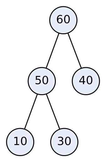
Max-heap after the five insertions
Extract-max: remove 60; move 30 to root → [30,50,40,10]; 30 < max(50,40)=50 → swap → [50,30,40,10]. Returned 60.
| Implementation | Insert | Delete (highest) |
|---|---|---|
| Unordered array | O(1) | O(n) |
| Ordered array | O(n) | O(1) |
| Sorted linked list | O(n) | O(1) |
| Binary heap | O(log n) | O(log n) |
3.7 Double-Ended Queue (Deque)
In one line: a deque (“deck”) is a queue where you can add and remove at both ends.
Understand it — a train with doors at both ends. Passengers can board or leave from the front door or the back door. It’s the most general linear list: use only one end and it’s a stack; use opposite ends and it’s a queue.
Definition
A deque (“deck”, Double Ended Queue) is a linear list in which insertion and deletion can be done at both ends — front and rear.
insert/delete ⇄ FRONT [ 10 | 20 | 30 | 40 ] REAR ⇄ insert/delete
Four operations: insertFront , insertRear , deleteFront , deleteRear (plus getFront, getRear, isEmpty, isFull).
Types of deque
-
Input-restricted deque: insertion at only one end (rear), deletion at both ends.
-
Output-restricted deque: deletion at only one end (front), insertion at both ends.
Input-restricted: delete ← [ ........ ] ← insert
 delete → (from rear too)
Output-restricted: delete ← [ ........ ] ← insert
 insert → (at front too)
| Input-restricted deque | Output-restricted deque |
|---|---|
| Insert: rear only | Insert: front and rear |
| Delete: front and rear | Delete: front only |
Deque as both stack and queue
As a stack: use insertRear + deleteRear only (same end) → LIFO.
As a queue: use insertRear + deleteFront (opposite ends) → FIFO.
Array implementation (circular)
insertFront(x): if full → overflow
 if F == −1: F = R = 0
 else F = (F − 1 + N) % N
 DQ[F] = x
insertRear(x): if full → overflow
 if F == −1: F = R = 0
 else R = (R + 1) % N
 DQ[R] = x
deleteFront(): if F == −1 → underflow
 x = DQ[F]
 if F == R: F = R = −1 else F = (F + 1) % N
deleteRear(): if F == −1 → underflow
 x = DQ[R]
 if F == R: F = R = −1 else R = (R − 1 + N) % N
full when: (R + 1) % N == F
Applications of deque: palindrome checking, undo/redo with limited history, sliding-window maximum, job-stealing schedulers, browser history.
3.8 Applications of Queues
-
CPU scheduling — round robin uses a circular queue of processes.
-
Printer spooling — print jobs served in order.
-
BFS (Breadth First Search) of graphs/trees uses a queue.
-
Buffers — keyboard buffer, I/O buffers, streaming (ring buffers).
-
Call centres / ticket systems — callers served in arrival order.
-
Network packet routing — routers queue packets.
-
Simulation of real-world waiting lines (banks, traffic).
-
Priority queues in Dijkstra, Huffman coding, OS task scheduling.
Linear Lists, Part C: Linked Lists
3.9 Linked List — the idea
Understand it first
Treasure-hunt analogy. Each clue (a node) has two things: a piece of the answer (the data) and directions to the next clue (the link/pointer). The clues can be hidden anywhere in the park — they don’t need to be next to each other. You only need to know where the first clue is (the HEAD). The last clue says “end” (NULL).
Compare with an array:
An array is like seats in a cinema row — numbered and side by side. You can jump straight to seat 7, but you can’t add a seat in the middle without shifting everyone. A linked list is like the treasure hunt — clues anywhere, joined by directions. Adding a new clue in the middle just means changing two directions; nothing moves. But to reach clue 7 you must follow clues 1 to 6.
So a linked list trades fast access for fast insertion/deletion and flexible size.
Arrays have a fixed size and costly insert/delete. A linked list solves both problems.
Definition: A linked list is a linear collection of data elements called nodes, where the linear order is given by pointers. Each node contains data and a link (pointer) to the next node. Nodes need not be contiguous in memory; memory is allocated dynamically.
Dynamic memory allocation in C (Lab practical 1)
| Dynamic memory allocation | in C (Lab practical 1) | |
|---|---|---|
| Function | Purpose | Example |
| malloc(size) | allocate size bytes; contents garbage; returns void* or NULL | p = (int*)malloc(5*sizeof(int)); |
| calloc(n, size) | allocate n blocks and set all to 0 | p = (int*)calloc(5, sizeof(int)); |
| realloc(p, newsize) | resize an earlier block | p = realloc(p, 10*sizeof(int)); |
| free(p) | release memory back to the heap | free(p); |
Memory for nodes comes from the heap; forgetting free causes a memory leak.
Array vs Linked list (7-mark question)
| Array vs Linked list (7-mark | question) | |
|---|---|---|
| Basis | Array | Linked list |
| Memory | Contiguous | Scattered, linked by pointers |
| Size | at Fixed compile time | at run Grows/shrinks time |
| Access | Random, O(1) by index | Sequential, O(n) |
| Insert/Delete | O(n) — shifting | O(1) once position known |
| Extra memory | None | One pointer per node (two for DLL) |
| Memory waste | Unused slots | No unused slots |
| Cache performance | Good (locality) | Poor |
| Binary search | Possible | Not practical |
Prefer array when size is known, frequent random access, binary search needed, memory tight. Prefer linked list when size unpredictable, frequent insertions/deletions in the middle, implementing stacks/queues/graphs (adjacency lists).
3.10 Singly Linked List (SLL)
In one line: each node has data + one pointer to the next node; you can only move forward.
How a node is stored: struct node groups an int data and a pointer next (the address of another struct node ). The program keeps a pointer head to the first node. head == NULL means the list is empty.
 HEAD
 │
 ▼
+----+---+ +----+---+ +----+---+ +----+------+
| 10 | ●─┼──▶| 20 | ●─┼──▶| 30 | ●─┼──▶| 40 | NULL |
+----+---+ +----+---+ +----+---+ +----+------+
 data next
Node structure in C:
struct node {
 int data; // information field
 struct node *next; // link field – address of next node
};
struct node *head = NULL; // empty list
HEAD/START pointer holds the address of the first node.
Last node’s next = NULL.
Empty list: head == NULL .
Creating a node
struct node* getnode(int x){
 struct node *p = (struct node*)malloc(sizeof(struct node));
 p->data = x; p->next = NULL; return p;
}
Traversal
Idea: start a temporary pointer p at head, process the node, move p to p->next , repeat until p becomes NULL. Never move head itself while traversing — you’d lose the start of the list forever.
Algorithm TRAVERSE(HEAD)
1. PTR ← HEAD
2. Repeat while PTR ≠ NULL
 Process PTR→DATA
 PTR ← PTR→NEXT
3. Exit
void display(){ struct node *p=head; while(p!=NULL){ printf("%d -> ",p->data); p=p->next;}
printf("NULL\n"); }
O(n). Counting nodes and searching use the same loop.
Insertion
The golden rule of linked-list insertion: first connect the new node to the rest of the list, then connect the previous node to the new node. If you do it the other way round, you overwrite the
only pointer to the rest of the list and lose it.
(a) At the beginning — O(1)
Algorithm INSERT_FIRST(HEAD, X)
1. NEW ← getnode() [allocate]
2. NEW→DATA ← X
3. NEW→NEXT ← HEAD [link new node to old first]
4. HEAD ← NEW [new node becomes first]
5. Exit
Before: HEAD → [10] → [20] → NULL
After : HEAD → [5] → [10] → [20] → NULL
void insFront(int x){ struct node *p=getnode(x); p->next=head; head=p; }
(b) At the end — O(n)
Algorithm INSERT_END(HEAD, X)
1. NEW ← getnode(); NEW→DATA ← X; NEW→NEXT ← NULL
2. If HEAD = NULL then HEAD ← NEW; Exit
3. PTR ← HEAD
4. Repeat while PTR→NEXT ≠ NULL: PTR ← PTR→NEXT
5. PTR→NEXT ← NEW
6. Exit
void insEnd(int x){ struct node *p=getnode(x),*t=head;
 if(!head){head=p;return;} while(t->next) t=t->next; t->next=p; }
(c) At a specified position POS (1-based) — O(n)
Algorithm INSERT_POS(HEAD, X, POS)
1. If POS = 1 then INSERT_FIRST; Exit
2. PTR ← HEAD; i ← 1
3. Repeat while i < POS − 1 and PTR ≠ NULL: PTR ← PTR→NEXT; i ← i + 1
4. If PTR = NULL then Write('Invalid position'); Exit
5. NEW ← getnode(); NEW→DATA ← X
6. NEW→NEXT ← PTR→NEXT
7. PTR→NEXT ← NEW
8. Exit
Order matters: step 6 before step 7, otherwise the rest of the list is lost.
(d) Insert in ascending (sorted) order (Lab practical 6c)
void insSorted(int x){
 struct node *p=getnode(x),*t;
 if(!head || x < head->data){ p->next=head; head=p; return; }
 t=head; while(t->next && t->next->data < x) t=t->next;
 p->next=t->next; t->next=p;
}
Deletion
Idea: to delete a node, make its previous node point past it (to its next), then free() it. For the first node, simply move head to the second node.
(a) Delete first node — O(1)
void delFirst(){ if(!head){printf("Underflow\n");return;}
 struct node *t=head; head=head->next; free(t); }
(b) Delete last node — O(n)
void delLast(){ if(!head) return;
 if(!head->next){ free(head); head=NULL; return; }
 struct node *t=head; while(t->next->next) t=t->next;
 free(t->next); t->next=NULL; }
(c) Delete node after a specified position / with a given key
Algorithm DELETE_KEY(HEAD, KEY)
1. If HEAD = NULL then Write('Underflow'); Exit
2. If HEAD→DATA = KEY then TEMP ← HEAD; HEAD ← HEAD→NEXT; free(TEMP); Exit
3. PREV ← HEAD; CUR ← HEAD→NEXT
4. Repeat while CUR ≠ NULL and CUR→DATA ≠ KEY: PREV ← CUR; CUR ← CUR→NEXT
5. If CUR = NULL then Write('Not found'); Exit
6. PREV→NEXT ← CUR→NEXT
7. free(CUR)
8. Exit
Reverse a singly linked list in place (7-mark)
Idea: walk through the list and turn every arrow around. You need three pointers: prev (the part already reversed), cur (the node being fixed), nxt (saves the rest of the list before we break cur ’s link).
Use three pointers: prev , cur , next .
void reverse(){
 struct node *prev=NULL, *cur=head, *nxt;
 while(cur){ nxt=cur->next; cur->next=prev; prev=cur; cur=nxt; }
 head=prev;
}
Trace on 1→2→3→NULL:
| Step | prev | cur | list state |
|---|---|---|---|
| start | NULL | 1 | 1→2→3 |
| 1 | 1 | 2 | NULL←1 2→3 |
| 2 | 2 | 3 | NULL←1←2 3 |
| 3 | 3 | NULL | NULL←1←2←3 |
| end | = head 3 | 3→2→1→NULL |
O(n) time, O(1) extra space.
Detect and remove a loop (Floyd’s cycle detection — 7-mark)
Use a slow pointer (1 step) and a fast pointer (2 steps). If they ever meet, there is a loop; if fast reaches NULL, no loop. To remove: put slow back at head; move both one step at a time; when slow->next == fast->next , set fast->next = NULL . (Special case: loop starts at head — then walk fast until fast->next == slow and cut.)
int detectAndRemove(){
 struct node *s=head,*f=head;
 while(f && f->next){ s=s->next; f=f->next->next; if(s==f) break; }
 if(!f || !f->next) return 0; // no loop
 s=head;
 if(s==f){ while(f->next!=s) f=f->next; }
 else { while(s->next!=f->next){ s=s->next; f=f->next; } }
 f->next=NULL; return 1;
}
Why it works: if the loop exists, the fast pointer gains one node per step and must catch the slow one inside the loop. O(n) time, O(1) space.
Merge two sorted lists (7-mark)
struct node* merge(struct node *a, struct node *b){
 struct node dummy, *t=&dummy; dummy.next=NULL;
 while(a && b){
 if(a->data <= b->data){ t->next=a; a=a->next; }
 else { t->next=b; b=b->next; }
 t=t->next;
 }
 t->next = a ? a : b;
 return dummy.next;
}
Trace: A = 1→4→7, B = 2→3→8 → compare 1,2 → take 1; 4,2 → 2; 4,3 → 3; 4,8 → 4; 7,8 → 7; A empty → attach 8. Result 1→2→3→4→7→8. O(m+n).
Advantages / disadvantages of SLL
✔ Dynamic size, easy insert/delete, no memory waste. ✘ Extra pointer memory, no random access, can only traverse forward, finding the previous node needs a scan.
3.11 Doubly Linked List (DLL)
In one line: each node has data + two pointers: prev (back) and next (forward), so you can move both ways.
Analogy: a train where every coach is connected to both the coach in front and the coach behind. You can walk forward or backward through the train.
Each node has two pointers: prev (to previous node) and next (to next node).
 +------+----+------+ +------+----+------+ +------+----+------+
NULL ◀────┼ prev | 10 | next ┼────▶┼ prev | 20 | next ┼────▶┼ prev | 30 | next ┼──▶ NULL
 +------+----+------+◀────┼──────+----+------+◀────┼──────+----+------+
 HEAD ▲ ▲ TAIL
struct dnode { struct dnode *prev; int data; struct dnode *next; };
struct dnode *head=NULL, *tail=NULL;
Advantage over SLL: traversal in both directions; deleting a node when you have a pointer to it is O(1) (you can reach its predecessor via prev ); easier insert-before. Disadvantage: extra pointer per node (more memory), more pointer updates per operation.
Insert at beginning
void dInsFront(int x){
 struct dnode *p=malloc(sizeof *p); p->data=x; p->prev=NULL; p->next=head;
 if(head) head->prev=p; else tail=p;
 head=p;
}
Insert at end
void dInsEnd(int x){
 struct dnode *p=malloc(sizeof *p); p->data=x; p->next=NULL; p->prev=tail;
 if(tail) tail->next=p; else head=p;
 tail=p;
}
Insert at position POS (after node T)
1. NEW→NEXT ← T→NEXT
2. NEW→PREV ← T
3. If T→NEXT ≠ NULL then T→NEXT→PREV ← NEW
4. T→NEXT ← NEW
Before: [A] ⇄ [B] After: [A] ⇄ [NEW] ⇄ [B]
Delete last node (5-mark)
Algorithm DELETE_LAST(HEAD, TAIL)
1. If HEAD = NULL then Write('Underflow'); Exit
2. TEMP ← TAIL
3. If HEAD = TAIL then HEAD ← TAIL ← NULL [only one node]
 Else TAIL ← TAIL→PREV; TAIL→NEXT ← NULL
4. free(TEMP)
5. Exit
(Without a tail pointer: traverse to the last node first.)
Delete node at position (pointer P to it)
1. If P→PREV ≠ NULL then P→PREV→NEXT ← P→NEXT else HEAD ← P→NEXT
2. If P→NEXT ≠ NULL then P→NEXT→PREV ← P→PREV else TAIL ← P→PREV
3. free(P)
Forward and backward traversal (Lab practical 8)
void forward(){ for(struct dnode *p=head;p;p=p->next) printf("%d ",p->data); }
void backward(){ for(struct dnode *p=tail;p;p=p->prev) printf("%d ",p->data); }
Applications of DLL: browser forward/back navigation, music player next/previous, undo-redo, LRU cache, deque implementation.
3.12 Circular Linked List (CLL)
In one line: the last node points back to the first instead of NULL, forming a ring.
Analogy: children sitting in a circle passing a parcel — after the last child, it goes back to the first. There’s no “end”.
Biggest trap: a loop like while (p != NULL) never stops on a circular list. You must stop when you get back to the starting node: do { … p = p->next; } while (p != head);
The last node points back to the first node instead of NULL. No node has a NULL link.
 ┌────────────────────────────────────────────┐
 ▼ │
 [10 | ●]──▶[20 | ●]──▶[30 | ●]──▶[40 | ●]───────┘
 HEAD/first LAST
Often only a pointer to the last node is kept, because last->next gives the first node — so insertion at both front and end is O(1).
Types: circular singly linked list and circular doubly linked list (last.next = first and first.prev = last).
Traversal (must stop when we return to start — not at NULL)
Algorithm CTRAVERSE(HEAD)
1. If HEAD = NULL then Write('Empty'); Exit
2. PTR ← HEAD
3. Repeat
 Process PTR→DATA
 PTR ← PTR→NEXT
 Until PTR = HEAD
4. Exit
void cdisplay(){ if(!head) return; struct node *p=head;
 do{ printf("%d ",p->data); p=p->next; } while(p!=head); }
Insert at end (with HEAD only)
void cInsEnd(int x){
 struct node *p=getnode(x);
 if(!head){ head=p; p->next=head; return; }
 struct node *t=head; while(t->next!=head) t=t->next;
 t->next=p; p->next=head;
}
Delete first node
void cDelFirst(){
 if(!head) return;
 if(head->next==head){ free(head); head=NULL; return; }
 struct node *t=head; while(t->next!=head) t=t->next; // find last
 struct node *old=head; head=head->next; t->next=head; free(old);
}
Convert a singly linked list into a circular linked list
Algorithm SLL_TO_CLL(HEAD)
1. If HEAD = NULL then Exit
2. PTR ← HEAD
3. Repeat while PTR→NEXT ≠ NULL: PTR ← PTR→NEXT [reach last node]
4. PTR→NEXT ← HEAD [link last to first]
5. Exit
Applications of CLL: round-robin CPU scheduling (processes take turns forever), multiplayer games (turn passing), circular buffers, repeating playlists, Josephus problem.
Comparison of SLL, DLL, CLL (5-mark)
| Comparison of SLL, | DLL, CLL (5-mark) | ||
|---|---|---|---|
| Basis | Singly | Doubly | Circular |
| Pointers per node | 1 (next) | 2 (prev, next) | 1 (or 2 if circular doubly) |
| Last node points to | NULL | NULL | First node |
| Traversal | Forward only | Forward & backward | Forward, endless loop from any node |
| Memory | Least | Most | Same as SLL |
| Delete given node | Need previous → O(n) | O(1) | Need previous → O(n) |
| End condition | p == NULL | p == NULL | p == head |
| Use | Simple lists, stacks | Navigation, LRU, deque | Round robin, buffers |
3.13 Linked Implementation of Stack (Lab practical 7)
Idea: treat the head of the list as the TOP. Push = insert at the front; pop = delete from the front. Both are O(1), and the stack can grow as long as memory lasts (no fixed MAX).
TOP is the head of the list; push = insert at front, pop = delete from front. No overflow (except when heap memory runs out).
struct node *top=NULL;
void push(int x){ struct node *p=getnode(x); p->next=top; top=p; }
int pop(){ if(!top){printf("Underflow\n");return -1;}
 struct node *t=top; int x=t->data; top=top->next; free(t); return x; }
push 10, 20, 30: TOP → [30] → [20] → [10] → NULL
pop → 30: TOP → [20] → [10] → NULL
3.14 Linked Implementation of Queue
Idea: keep two pointers — front (delete here) and rear (insert here). Enqueue adds after rear ; dequeue removes at front . Both O(1).
Keep FRONT (delete here) and REAR (insert here).
struct node *front=NULL,*rear=NULL;
void enqueue(int x){ struct node *p=getnode(x);
 if(!rear){ front=rear=p; return; } rear->next=p; rear=p; }
int dequeue(){ if(!front){printf("Underflow\n");return -1;}
 struct node *t=front; int x=t->data; front=front->next;
 if(!front) rear=NULL; free(t); return x; }
Both operations O(1). No overflow, no wasted space.
Circular queue using a singly linked list: keep only rear ; rear->next is the front. enqueue: new node p; if empty, p->next = p ; else p->next = rear->next; rear->next = p ; then rear = p . dequeue: f = rear->next ; if f == rear the queue becomes empty; else rear->next = f->next ; free f.
Priority queue using a linked list: keep nodes sorted by priority; insert walks to the correct position O(n); delete removes the head O(1). Compare with heap: O(log n) for both.
3.15 Applications of Linked Lists
-
Implementing stacks, queues, deques, priority queues.
-
Polynomial representation and arithmetic — each node = (coefficient, exponent, next). 5𝑥3 + 4𝑥2 + 2 → [5,3] → [4,2] → [2,0] → NULL . Adding two polynomials = merging two lists by exponent.
-
Adjacency lists for graphs.
-
Sparse matrices (store only non-zero elements).
-
Dynamic memory management (free lists in OS).
-
Undo functionality, browser history (DLL), music playlists (CLL).
-
Hash table chaining (collision resolution).
-
Representing very long integers (digit per node).
Unit 3 — What to write in the exam (question bank map)
3-mark: Define stack/queue/deque/priority queue. Overflow & underflow conditions. Input- vs output-restricted deque. SLL node structure in C. Linear vs circular queue (memory). Advantages of linked list over array. DLL advantage over SLL. CLL application. 5-mark: PUSH/POP algorithms; enqueue/dequeue for linear and circular queue; deque types with
diagram; priority queue using array and its limitations; insert at beginning of SLL; delete last node of DLL; traverse CLL; compare SLL/DLL/CLL; stack & queue from one deque; min- heap priority queue. 7-mark: Convert infix → postfix with table (e.g., A+(B*C−(D/E^F)*G)*H → A B C * D E F ^ / G * − H * + ); evaluate postfix; complete linear and circular queue with trace; deque with all four operations; max-heap PQ trace; SLL insertion at
beginning/end/position; DLL insert/delete at position; SLL→CLL; reverse SLL; detect & remove loop; merge two sorted lists; array vs linked list; queue applications.
Unit 3 — Common mistakes
Stack: checking overflow after incrementing TOP (must check first).
Postfix evaluation: popping the operands in the wrong order for − and /.
Circular queue: writing rear + 1 instead of (rear + 1) % N .
Linked list insertion: changing prev->next before setting new->next (loses the rest of the list).
Circular list traversal using while (p != NULL) (infinite loop).
Forgetting the empty-list and single-node special cases.
Unit 3 — Check yourself
-
Queue of size 5 using an array: after inserting 1, 2, 3, 4, 5 and deleting twice, can a linear queue accept a new element? A circular one?
-
In a circular queue with N = 6, F = 4, R = 3 — is it full?
-
Write the two pointer statements to insert node N after node P in an SLL.
-
Which linked list lets you delete a node in O(1) when you have a pointer to it?
-
Max-heap [60, 50, 40, 10, 30] — after extract-max?
Answers: 1) Linear: no (REAR = N − 1 → overflow); circular: yes (REAR wraps to 0). 2) (3 + 1) % 6 = 4 = F → full. 3) N->next = P->next; P->next = N; . 4) Doubly linked list. 5) [50, 30, 40, 10].
Non-Linear Lists: Trees
4.1 Tree — definition and terminology
Understand it first
Until now every structure was a line. But lots of real information is hierarchical — it branches:
your family tree (grandparents → parents → children),
folders on your computer (C: → Users → maher → Downloads → files),
a company org chart (CEO → managers → employees).
A tree stores exactly this kind of data. Computer scientists draw trees upside down: the root at the top, branches going down, leaves at the bottom.
A tree is a non-linear, hierarchical data structure consisting of a finite set of nodes connected by edges, such that:
-
There is one special node called the root.
-
The remaining nodes are partitioned into disjoint subsets, each of which is itself a tree (a subtree of the root).
A tree with n nodes always has n − 1 edges and no cycles.
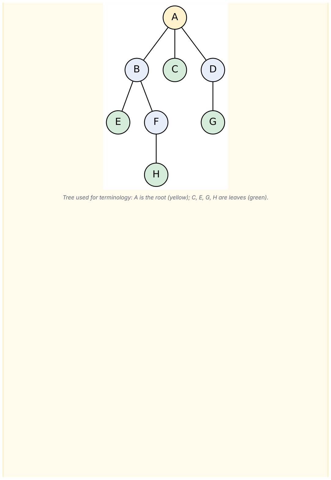
| Term | Meaning (with the tree above) |
|---|---|
| Node | Element holding data (A … H) |
| Root | Topmost node, no parent (A) |
| Edge | Link between parent and child (A–B) |
| Parent | Node with a branch to a lower node (B is parent of E, F) |
| Child | Node directly below a parent F are children of (E, B) |
| Siblings | Children of the same parent (B, C, D) |
| Leaf / terminal / external node | Node with no children (E, H, C, G) |
| Internal / non-terminal node | Node with at least one child (A, B, D, F) |
| Degree of a node | Number of children (deg A = 3, deg B = 2, deg E = 0) |
| Degree of tree | Maximum degree of any node (3) |
| Level | Root at level 0; children at parent level + 1 (H at level 3) |
| Depth of a node | Number of edges from root to that node (depth F = 2) |
| Height of a node | Number of edges on the longest path from it down to a leaf (height B = 2) |
| Height of tree | Height of root = maximum level (3) |
| Path | Sequence of nodes connected by edges (A–B–F– H) |
| Ancestor | Any node on the path from root to that node (A, B, F are ancestors of H) |
| Descendant | Any node in its subtree (E, F, H are descendants of B) |
| Subtree | A node together with all its descendants |
A set of disjoint trees (remove the root → forest) Forest
4.2 Binary Tree
In one line: a tree where every node has at most two children, called left and right.
The “left” and “right” positions matter: a node with only a left child is a different binary tree from a node with only a right child.
A binary tree is a tree in which each node has at most two children, called the left child and the right child (order matters). A binary tree can also be empty.
Types of binary trees
| Type | Definition |
|---|---|
| Strictly (full/proper) binary tree | Every node has 0 or 2 children |
| Complete binary tree | All levels full except possibly the last, which is filled left to right |
| Perfect binary tree | All internal nodes have 2 children and all leaves at the same level |
| Skewed binary tree | Every node has only one child (left-skewed or right- a skewed) — behaves like linked list |
| Extended binary tree (2-tree) | a Replace every empty subtree with special external node; all original nodes then have 2 children |
 Strict: A Complete: A Left-skewed: A
 / \ / \ /
 B C B C B
 / \ / \ /
 D E D E C
Properties (memorise)
-
Maximum nodes at level i = 2ⁱ.
-
Maximum nodes in a binary tree of height h = 2^(h+1) − 1.
-
Minimum height of a binary tree with n nodes = ⌈log₂(n+1)⌉ − 1.
-
In any non-empty binary tree, n₀ = n₂ + 1 (leaves = nodes with 2 children + 1).
-
A tree with n nodes has n − 1 edges; a binary tree with n nodes has n+1 NULL links.
4.3 Representation of a Binary Tree
(a) Array (sequential) representation
Store nodes level by level. With 0-based index i:
left child at 2i + 1, right child at 2i + 2, parent at ⌊(i − 1)/2⌋.
With 1-based index i: left = 2i, right = 2i + 1, parent = ⌊i/2⌋.
 A index: 0 1 2 3 4 5 6
 / \ value: A B C D E - F
 B C
 / \ \
 D E F
✔ Simple, no pointers, good for complete trees (heaps). ✘ Wastes space for skewed/sparse trees (a right-skewed tree of height h needs 2^(h+1)−1 slots), fixed size.
(b) Linked representation
struct tnode {
 struct tnode *left;
 int data;
 struct tnode *right;
};
 / \
 [ ● | B | ● ] [NULL| C | ● ]
 / \ \
[NULL|D|NULL] [NULL|E|NULL] [NULL|F|NULL]
✔ No wasted space, dynamic size, easy insert/delete. ✘ Extra memory for pointers; n + 1 pointers are NULL (wasted — threaded trees use them).
4.4 Tree Traversals
Understand it first
Traversal = visiting every node exactly once (to print them, count them, search them). In a list there is only one natural order; in a tree you must decide when to visit the node itself relative to its two subtrees. That gives three orders — the name tells you where the root (N) goes:
Preorder = root before the subtrees: N L R
Inorder = root in between: L N R
Postorder = root after the subtrees: L R N
The left subtree is always done before the right one. Each subtree is traversed with the same rule, recursively.
Trick for doing it by hand: draw a line hugging the tree, starting left of the root and going around counter-clockwise. Write a node when you pass its left side (preorder), its bottom (inorder), or its right side (postorder).
Traversal = visiting every node exactly once. Three depth-first orders (L = left subtree, N = node/root, R = right subtree):
| R = right | subtree): | |
|---|---|---|
| Traversal | Order | Mnemonic |
| Preorder | N L R | root first |
| Inorder | L N R | root in the middle |
| Postorder | L R N | root last |
| Level order | level by level, left to right (uses a queue) | BFS |
Recursive algorithms
void preorder(struct tnode *t){ if(t){ printf("%d ",t->data); preorder(t->left); preorder(t-
>right);} }
void inorder(struct tnode *t){ if(t){ inorder(t->left); printf("%d ",t->data); inorder(t-
>right);} }
void postorder(struct tnode *t){ if(t){ postorder(t->left); postorder(t->right); printf("%d
",t->data);} }
Worked example
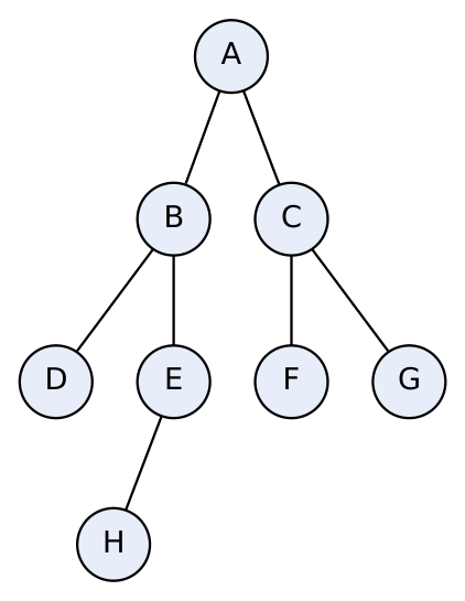
Example tree for traversals
Preorder: A B D E H C F G
Inorder: D B H E A F C G
Postorder: D H E B F G C A
Level order: A B C D E F G H
Expression tree: for (a + b) * (c − d) :
 *
 / \
 + −
 / \ / \
 a b c d
Preorder = * + a b − c d (prefix), Inorder = a + b * c − d (infix), Postorder = a b + c d − * (postfix).
Non-recursive (iterative) traversals using a stack (Lab practical 10b)
Inorder:
1. Initialise empty stack S; PTR ← ROOT
2. Repeat while PTR ≠ NULL or S not empty
 a. While PTR ≠ NULL: push PTR; PTR ← PTR→LEFT [go as left as possible]
 b. PTR ← pop(S); visit PTR
 c. PTR ← PTR→RIGHT
Preorder:
1. If ROOT = NULL exit; push ROOT
2. While S not empty: PTR ← pop; visit PTR;
 if PTR→RIGHT push it; if PTR→LEFT push it [right first so left is
processed first]
Postorder (two stacks): push root on S1; repeatedly pop from S1, push it on S2, push its left then right onto S1. Finally pop all of S2 → postorder.
Constructing a binary tree from traversals
A unique binary tree can be built from Inorder + Preorder or Inorder + Postorder (not from Pre + Post alone).
Example: Preorder: A B D E C F; Inorder: D B E A F C.
-
First of preorder = root = A. In inorder, left of A = {D, B, E} (left subtree), right = {F, C}.
-
Next in preorder = B → root of left subtree; inorder left of B = D, right = E.
-
Next = C → root of right subtree; inorder left of C = F.
 A
 / \
 B C
 / \ /
 D E F
4.5 Threaded Binary Tree
Understand it first
In a normal linked binary tree, every leaf has two NULL pointers — in a tree of n nodes, n + 1 pointers are wasted. Also, doing an inorder traversal needs recursion or a stack to “come back up”.
Idea: reuse those empty pointers as shortcuts (threads): an empty right pointer points to the node that comes next in inorder (inorder successor); an empty left pointer points to the node that comes before in inorder (inorder predecessor). Then you can walk through the tree in inorder just by following pointers — no stack, no recursion.
Problem: a linked binary tree with n nodes has n + 1 NULL pointers — wasted. Also, inorder traversal needs recursion or a stack.
Idea (A. J. Perlis & C. Thornton): replace NULL pointers with threads — pointers to the inorder predecessor (in a NULL left link) or inorder successor (in a NULL right link).
Right-threaded (one-way): NULL right link → inorder successor.
Left-threaded: NULL left link → inorder predecessor.
Fully threaded (two-way): both.
To tell a thread from a real child, each node has two flag bits:
struct tbnode {
 int lthread; // 1 = left is a thread, 0 = real child
 struct tbnode *left;
 int data;
 struct tbnode *right;
 int rthread; // 1 = right is a thread
};
Example: inorder of the tree below is D B E A C.
 A
 / \
 B C
 / \
 D E
Threads (dotted): D.left → (header / NULL), D.right → B
 E.left → B, E.right → A
 C.left → A, C.right → (header / NULL)
Often a header (dummy) node is used so the first node’s left thread and last node’s right thread point to it instead of NULL.
Inorder traversal without stack:
1. PTR ← leftmost node of the tree
2. Repeat while PTR ≠ NULL (or header)
 visit PTR
 If PTR→rthread = 1 then PTR ← PTR→RIGHT [follow thread to successor]
 Else PTR ← leftmost node in PTR→RIGHT subtree
Advantages: inorder traversal is faster with no stack/recursion; finding inorder
successor/predecessor is easy; uses the NULL links. Disadvantages: insertion/deletion are more complex; extra flag bits per node.
4.6 Binary Search Tree (BST)
Understand it first
The number-guessing game again. At each node you ask “is my key smaller or bigger than this?” and go left or right — throwing away half the remaining tree each time (if the tree is balanced). That’s why a BST search is O(log n), like binary
search, but insertion and deletion are also fast (no shifting, unlike a sorted array).
The BST rule: smaller keys go left, larger keys go right — at every node, not just the root.
A BST is a binary tree where for every node:
all keys in its left subtree are smaller than the node’s key,
all keys in its right subtree are greater,
both subtrees are also BSTs (duplicates usually not allowed).
Key property: Inorder traversal of a BST gives keys in ascending order.
Construct a BST — insert 50, 30, 70, 20, 40, 60, 80, 35
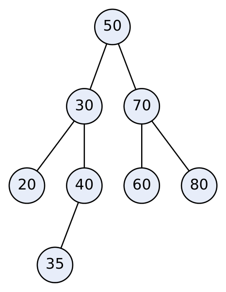
BST after inserting 50, 30, 70, 20, 40, 60, 80, 35
Inorder: 20 30 35 40 50 60 70 80 (sorted ✔).
Search
Algorithm BST_SEARCH(ROOT, KEY)
1. PTR ← ROOT
2. Repeat while PTR ≠ NULL
 If KEY = PTR→DATA then Return PTR [found]
 Else if KEY < PTR→DATA then PTR ← PTR→LEFT
 Else PTR ← PTR→RIGHT
3. Return NULL [not found]
Insert (Lab practical 10a)
struct tnode* insert(struct tnode *t, int key){
 if(t==NULL){ t=malloc(sizeof *t); t->data=key; t->left=t->right=NULL; return t; }
 if(key < t->data) t->left = insert(t->left, key);
 else if(key > t->data) t->right = insert(t->right, key);
 return t;
}
Delete — three cases
Why is two-children the hard case? You can’t just remove the node — it has two subtrees that both need a parent. So you replace its value by a value that keeps the BST rule true: the smallest value in its right subtree (inorder successor) — it’s bigger than everything on the left
and smaller than everything else on the right. That successor node has no left child, so removing it is an easy case (0 or 1 child).
-
Leaf node: simply remove it (set parent’s link to NULL). Delete 35.
-
One child: replace the node by its child. Delete 40 (after 35 removed it has none; suppose 40 has child 35 → link 30’s right to 35).
-
Two children: replace the node’s key with its inorder successor (smallest key in right subtree) — or inorder predecessor — then delete that successor (which has at most one child). Delete 50 → successor is 60 → root becomes 60; remove old 60.
Delete 50 from the tree above: 60
 / \
 30 70
 / \ \
 20 40 80
 /
 35
struct tnode* minNode(struct tnode *t){ while(t->left) t=t->left; return t; }
struct tnode* del(struct tnode *t, int key){
 if(!t) return t;
 if(key < t->data) t->left = del(t->left, key);
 else if(key > t->data) t->right = del(t->right, key);
 else {
 if(!t->left){ struct tnode *r=t->right; free(t); return r; }
 if(!t->right){ struct tnode *l=t->left; free(t); return l; }
 struct tnode *s = minNode(t->right);
 t->data = s->data;
 t->right = del(t->right, s->data);
 }
 return t;
}
Complexity: search/insert/delete = O(h). Balanced tree h ≈ log n → O(log n); skewed tree (inserting sorted data 10,20,30,…) h = n → O(n).
Applications of BST: dictionaries / symbol tables, database indexing, sorting (tree sort), set/map implementations, range queries.
4.7 Conversion of a General Tree to a Binary Tree
Understand it first
A general tree can have any number of children per node, which is awkward to store (how many pointers should each node have?). The trick: every node needs only two pointers — one to its eldest (first) child, one to its next younger sibling. That is exactly a binary tree. Left = first child, Right = next sibling (LCRS).
A general tree can have any number of children. It is converted to a binary tree using the Left-Child Right-Sibling (LCRS) rule (Knuth transformation):
-
The root of the binary tree = root of the general tree.
-
Left pointer of each node → its first (leftmost) child.
-
Right pointer of each node → its next sibling (immediate right brother).
-
Remove all other parent–child edges.
(Visual trick: link all siblings horizontally, keep only the edge from each parent to its leftmost child, then rotate the picture 45° clockwise.)
General tree
Binary tree (left = first child, right = next sibling)
Example:
Explanation: A’s first child B → A.left = B. B’s next sibling C → B.right = C; C’s next sibling D → C.right = D. B’s first child E → B.left = E; E’s sibling F → E.right = F. D’s first child G → D.left = G.
Note: the root of the converted binary tree never has a right child (the root has no siblings). Preorder of the binary tree = preorder of the general tree.
Forest → binary tree: convert each tree, then link the roots of the trees as right siblings of each other.
4.8 Applications of trees
File systems (folders), HTML DOM, organisation charts, expression trees (compilers), BSTs for searching, heaps for priority queues, Huffman coding trees (compression), decision trees (AI), B-trees (database indexes), routing tables, syntax/parse trees.
Unit 4 — Exam Questions You Must Be Able to Answer
-
Define tree and explain terminology (root, leaf, degree, level, height, depth, sibling) with a diagram.
-
Define binary tree; types (strict, complete, skewed); properties (2ⁱ, 2^(h+1)−1, n₀ = n₂+1).
-
Array vs linked representation of a binary tree.
-
Give preorder, inorder, postorder (and level order) for a given tree. Write recursive and non- recursive algorithms.
-
Construct a binary tree from inorder + preorder/postorder.
-
What is a threaded binary tree? Why is it needed? Draw threads for a given tree; write inorder traversal.
-
Construct a BST from a sequence; delete nodes (all three cases); show inorder.
-
Convert a general tree to a binary tree.
Unit 4 — Common mistakes
Visiting the right subtree before the left.
In postorder, writing the root before finishing both subtrees.
BST: comparing only with the root (the rule applies at every node).
Two-children delete: using the inorder successor from the left subtree (it must be the smallest in the right subtree, or the largest in the left — the predecessor).
General → binary: making the second child a left child (siblings always go right).
Unit 4 — Check yourself
- Max nodes in a binary tree of height 3? 2. Inorder of a BST built from 15, 10, 20, 8, 12? 3. Preorder A B D E C F and inorder D B E A F C — draw the tree. 4. Why is a threaded tree useful?
Answers: 1) 2⁴ − 1 = 15. 2) 8 10 12 15 20. 3) A(B(D, E), C(F, –)). 4) Inorder traversal without a
stack/recursion, using the n + 1 empty pointers.
Graphs
5.1 Definition
Understand it first
A tree has a strict parent–child hierarchy. A graph has no such rule: anything can connect to anything.
Google Maps: cities are vertices, roads are edges (with distances as weights).
Instagram: people are vertices, “follows” are directed edges (you may follow someone who doesn’t follow you).
Facebook friends: undirected edges (friendship works both ways).
A tree is just a special graph: connected and with no cycles.
A graph G = (V, E) is a non-linear data structure consisting of
V — a finite, non-empty set of vertices (nodes), and
E — a set of edges, each connecting a pair of vertices.
Unlike a tree, a graph can have cycles, need not have a root, and any vertex can connect to any other. A tree is a special graph (connected and acyclic).
A B C D
Example graph
V = {A, B, C, D}, E = {(A,B), (A,C), (B,C), (B,D), (C,D)}
5.2 Graph Terminologies
| Term | Meaning |
|---|---|
| Vertex / node | A point in the graph |
| Edge / arc | A connection between two vertices |
| Undirected graph | Edges have no direction: (u, v) = (v, u) |
| Directed graph (digraph) | Each edge has a direction: ⟨u, v⟩ goes from u (tail) to v (head) |
| Weighted graph (network) | Each edge carries a weight/cost (distance, time) |
| Adjacent vertices (neighbours) | Two vertices joined by an edge |
| Incident edge | Edge (u, v) is incident on u and v |
| Degree (undirected) | Number of edges incident on a vertex |
| In-degree / Out-degree (directed) | Number of edges coming in / going out |
| Source / Sink | Vertex with in-degree 0 / out-degree 0 |
| Isolated vertex | Degree 0 |
| Pendant vertex | Degree 1 |
| Path | Sequence of vertices where each consecutive pair is adjacent |
| Simple path | Path with no repeated vertices |
| Path length | Number of edges on the path |
| Cycle | Path that starts and ends at the same vertex (length ≥ 3 in undirected) |
| Acyclic graph | No cycles; directed acyclic graph = DAG |
| Self-loop | Edge from a vertex to itself |
| Parallel / multiple edges | More than one edge between the same pair → multigraph |
| Simple graph | No no self-loops and parallel edges |
| Connected graph | A path exists between every pair of vertices (undirected) |
| Strongly connected | Directed: path from every u to every v and back |
| Weakly connected | Directed graph connected when directions are ignored |
Complete graph Kₙ
Every pair of vertices is joined; has n(n−1)/2 edges
| Term | Meaning |
|---|---|
| Subgraph | G’ = (V’, E’) with V’ ⊆ V, E’ ⊆ E |
| Spanning tree | a Subgraph that is tree and includes all vertices (n−1 |
| edges) | |
| Connected component | Maximal connected subgraph |
| Dense / sparse | Many edges (≈ n²) / few edges (≈ n) |
Handshaking lemma: Sum of degrees of all vertices = 2 × number of edges. (So the number of odd-degree vertices is always even.) For a digraph: Σ in-degree = Σ out-degree = |E|.
5.3 Representation of Graphs
A computer can’t “see” a drawing, so we must store the graph as data. Two standard ways:
Adjacency matrix — a table: “is there a road from city i to city j?” (yes = 1, no = 0). Adjacency list — for each city, a list of the cities directly connected to it.
(a) Adjacency Matrix
For a graph with n vertices, an n × n matrix A where
𝐴[ 𝑖] [ 𝑗] = { 1
if there is an edge from 𝑖to 𝑗
0
otherwise
For a weighted graph store the weight instead of 1 (and 0 or ∞ for no edge).
Undirected example (graph in 5.1, A=0, B=1, C=2, D=3):
| example | (graph in 5.1, A=0, | B=1, C=2, D=3): | ||
|---|---|---|---|---|
| A | B | C | D | |
| A | 0 | 1 | 1 | 0 |
| B | 1 | 0 | 1 | 1 |
| C | 1 | 1 | 0 | 1 |
| D | 0 | 1 | 1 | 0 |
Undirected → matrix is symmetric; row sum = degree.
Directed → not necessarily symmetric; row sum = out-degree, column sum = in-degree.
Directed example: edges 1→2, 1→3, 2→4, 3→4, 4→1
| 1 | 2 | 3 | 4 | |
|---|---|---|---|---|
| 1 | 0 | 1 | 1 | 0 |
| 2 | 0 | 0 | 0 | 1 |
| 3 | 0 | 0 | 0 | 1 |
| 4 | 1 | 0 | 0 | 0 |
✔ Edge check O(1); simple. ✘ Space O(V²) even for sparse graphs; finding all neighbours O(V).
(b) Adjacency List
An array of n linked lists; list i contains all vertices adjacent to vertex i.
A → B → C → NULL
B → A → C → D → NULL
C → A → B → D → NULL
D → B → C → NULL
struct anode { int vertex; struct anode *next; };
struct anode *adj[MAX]; // adj[i] = head of list for vertex i
Undirected graph: total list nodes = 2E. Directed: E.
✔ Space O(V + E) — good for sparse graphs; neighbours listed quickly. ✘ Checking whether edge (u,v) exists is O(degree(u)).
| Basis | Adjacency matrix | Adjacency list |
|---|---|---|
| Space | O(V²) | O(V + E) |
| Check edge (u,v) | O(1) | O(deg u) |
| Find all neighbours | O(V) | O(deg u) |
| Add edge | O(1) | O(1) |
| Best for | Dense graphs | Sparse graphs |
| DFS/BFS time | O(V²) | O(V + E) |
(Other representations: incidence matrix — V × E; edge list.)
5.4 Elementary Graph Operations — Traversal

Understand it first
DFS (Depth-First Search) — like exploring a maze: keep going forward along one corridor as deep as you can; when you hit a dead end, back up to the last junction and try another corridor. Uses a stack (recursion does this automatically).
BFS (Breadth-First Search) — like ripples in a pond or news spreading: first visit all places 1 step away, then all places 2 steps away, and so on. Uses a queue. Because it goes level by level, BFS finds the shortest path (fewest edges).
Both need a visited[] array — graphs can have cycles, and without it you’d go round a cycle forever.
Traversal = visiting every vertex reachable from a start vertex exactly once. A visited[] array prevents visiting a vertex twice (graphs can have cycles).
Depth First Search (DFS)
Idea: go as deep as possible along one path before backtracking. Uses a stack (explicitly, or implicitly through recursion).
Algorithm DFS(v)
1. visited[v] ← TRUE; visit v
2. For each vertex w adjacent to v
 If visited[w] = FALSE then DFS(w)
Iterative:
1. Push start vertex S onto stack
2. Repeat while stack not empty
 a. v ← pop
 b. If v not visited: mark visited, visit v,
 push all unvisited neighbours of v (in reverse order so the smallest is processed
first)
Breadth First Search (BFS)
Idea: visit the start vertex, then all its neighbours, then their neighbours — level by level. Uses a queue.
Algorithm BFS(s)
1. visited[s] ← TRUE; enqueue(s)
2. Repeat while queue not empty
 a. v ← dequeue; visit v
 b. For each vertex w adjacent to v
 If visited[w] = FALSE then visited[w] ← TRUE; enqueue(w)
Worked example (neighbours taken in alphabetical order)
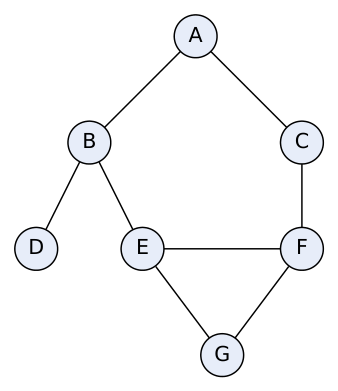
Graph used for the DFS/BFS example
Adjacency lists: A: B,C | B: A,D,E | C: A,F | D: B | E: B,F,G | F: C,E,G | G: E,F
DFS from A (recursive): A → B (first unvisited neighbour of A) → D (B’s first unvisited) → D has no unvisited → back to B → E → F (E’s first unvisited after B) → C (F’s first unvisited) → C has none → back to F → G → done. DFS order: A B D E F C G
BFS from A:
| from | A: | ||
|---|---|---|---|
| Step | Dequeue | Enqueue (unvisited neighbours) | Queue after |
| 0 | – | A | A |
| 1 | A | B, C | B C |
| 2 | B | D, E | C D E |
| 3 | C | F | D E F |
| 4 | D | – | E F |
| 5 | E | G | F G |
| 6 | F | – | G |
| 7 | G | – | empty |
BFS order: A B C D E F G
C program — DFS and BFS on adjacency matrix (Lab practical 13)
#include <stdio.h>
int n, a[10][10], visited[10];
void dfs(int v){
 visited[v]=1; printf("%d ", v);
 for(int w=0; w<n; w++)
 if(a[v][w] && !visited[w]) dfs(w);
}
void bfs(int s){
 int q[10], f=0, r=0;
 for(int i=0;i<n;i++) visited[i]=0;
 visited[s]=1; q[r++]=s;
 while(f<r){
 int v=q[f++]; printf("%d ", v);
 for(int w=0; w<n; w++)
 if(a[v][w] && !visited[w]){ visited[w]=1; q[r++]=w; }
 }
}
int main(){
 scanf("%d",&n);
 for(int i=0;i<n;i++) for(int j=0;j<n;j++) scanf("%d",&a[i][j]);
 dfs(0); printf("\n"); bfs(0);
}
DFS vs BFS
| Basis | DFS | BFS |
|---|---|---|
| Data structure | Stack (or recursion) | Queue |
| Strategy | Go deep, then backtrack | Level by level |
| Shortest path (unweighted) | Not guaranteed | Guaranteed (fewest edges) |
| Memory | O(depth) | O(width) — can be large |
| Produces | DFS spanning tree | BFS spanning tree |
| Time | O(V+E) list / O(V²) matrix | O(V+E) list / O(V²) matrix |
| Uses | Cycle detection, topological sort, connected components, maze solving, path existence | Shortest path in unweighted graphs, web crawlers, social network “friends within k”, peer- to-peer networks, GPS neighbours |
5.5 Applications of Graphs
Maps & navigation: cities = vertices, roads = weighted edges (shortest path — Dijkstra). Social networks: people = vertices, friendships = edges (friend suggestions via BFS). Computer networks / Internet routing.
Web: pages = vertices, hyperlinks = directed edges (search engines, PageRank).
Dependency resolution / scheduling: DAG + topological sort (course prerequisites, build systems).
Electric circuits, molecule structures, recommendation systems.
Minimum spanning tree (Prim, Kruskal) for cheapest network/cable layout.
Unit 5 — Exam Questions You Must Be Able to Answer
-
Define graph; explain terminologies (directed, undirected, weighted, degree, in/out-degree, path, cycle, connected, complete graph) with diagrams.
-
Represent a given graph by adjacency matrix and adjacency list; compare them.
-
Explain DFS with algorithm and give the DFS order for a given graph.
-
Explain BFS with algorithm, show queue contents step by step.
-
Differentiate DFS and BFS. Applications of graphs.
Unit 5 — Common mistakes
Forgetting the visited check (infinite loop on a cycle).
In BFS, marking a vertex visited when dequeued instead of when enqueued (it may then be enqueued twice).
Writing an undirected adjacency matrix that isn’t symmetric.
Unit 5 — Check yourself
- A graph has 5 vertices with degrees 3, 2, 2, 2, 1. How many edges? 2. Space for an adjacency matrix of 100 vertices? 3. Which traversal finds the fewest-edge path? 4. Complete graph with 6 vertices — edges?
Answers: 1) Σdeg/2 = 10/2 = 5. 2) 100 × 100 = 10,000 entries. 3) BFS. 4) 6 × 5 / 2 = 15.
Searching & Sorting
6.1 Basics
Searching: finding whether a given element (key) is present in a collection and, if so, its position. Sorting: arranging elements in a particular order (ascending/descending).
Sorting terms:
Internal sort: all data fits in main memory (RAM) — bubble, selection, insertion, quick. External sort: data too large for RAM, kept on disk/tape — external merge sort.
Stable sort: equal keys keep their original relative order (bubble, insertion, merge: stable; selection, quick: not stable).
In-place: needs only O(1) extra memory (bubble, selection, insertion, quick*).
Pass: one complete scan over the (unsorted part of the) list.
Classification by technique (as in the syllabus): selection sorts (selection, heap), insertion sorts (insertion, shell), exchange sorts (bubble, quick), merge sorts (merge, external).
6.2 Linear (Sequential) Search
In one line: check every element one by one from the start until you find the key or reach the end.
Like finding your friend in a crowd when you have no idea where they are — you look at each face in turn. Works on any list, sorted or not.
Compare the key with each element from the first to the last until found or the list ends. Works on unsorted data.
Algorithm LINEAR_SEARCH(A, N, KEY)
1. Repeat for I ← 0 to N − 1
 If A[I] = KEY then Return I [found at I]
2. Return −1 [not found]
int linearSearch(int a[], int n, int key){
 for(int i=0;i<n;i++) if(a[i]==key) return i;
 return -1;
}
Example: A = [7, 3, 9, 1, 5], key = 1 → comparisons with 7, 3, 9, 1 → found at index 3 (4 comparisons).
Complexity: best O(1), average (n+1)/2 → O(n), worst O(n). ✔ Simple, unsorted data, linked lists. ✘ Slow for large n.
Sentinel search: place the key at A[n] so the loop needs no bounds check — saves one comparison per step.
6.3 Binary Search
In one line: in a sorted list, look at the middle; if the key is smaller, throw away the right half, otherwise the left half; repeat.
Dictionary analogy: looking up “Maher”, you open the middle (“K”), see M comes after K, and ignore the whole first half. Each look halves the pages left. 1000 pages → at most 10 looks. It only works if the data is sorted — otherwise “smaller → go left” means nothing.
Works only on a sorted array. Compare the key with the middle element; if smaller, search the left half; if larger, the right half. Each comparison halves the search space (divide and conquer).
Algorithm BINARY_SEARCH(A, N, KEY)
1. LOW ← 0; HIGH ← N − 1
2. Repeat while LOW ≤ HIGH
 MID ← ⌊(LOW + HIGH) / 2⌋
 If KEY = A[MID] then Return MID
 Else if KEY < A[MID] then HIGH ← MID − 1
 Else LOW ← MID + 1
3. Return −1
int binarySearch(int a[], int n, int key){
 int lo=0, hi=n-1;
 while(lo<=hi){
 int mid=lo+(hi-lo)/2; // avoids overflow
 if(a[mid]==key) return mid;
 else if(key<a[mid]) hi=mid-1;
 else lo=mid+1;
 }
 return -1;
}
Trace: A = [5, 12, 17, 23, 38, 44, 77, 84, 90], key = 77 (n = 9)
| Iter | LOW | HIGH | MID | A[MID] | Action |
|---|---|---|---|---|---|
| 1 | 0 | 8 | 4 | 38 | 77 > 38 → LOW = 5 |
| 2 | 5 | 8 | 6 | 77 | found at index 6 |
Key = 20: (0,8,4: 38 → HIGH=3), (0,3,1: 12 → LOW=2), (2,3,2: 17 → LOW=3), (3,3,3: 23 → HIGH=2), LOW > HIGH → not found.
Complexity: best O(1), average and worst O(log₂ n). Max comparisons for n elements = ⌊log₂ n⌋ + 1. (e.g., 35 elements → at most 6 comparisons; 1,000,000 elements → 20.)
| 1. (e.g., 35 elements → at most 6 comparisons; 1,000,000 | elements → 20.) |
|---|---|
| Linear search | Binary search |
| or Unsorted sorted data | Sorted data only |
| OK Sequential access (linked list) | Needs random access (array) |
| O(n) | O(log n) |
| Simple | Slightly complex |
6.4 Bubble Sort (Exchange sort)
In one line: repeatedly walk through the list swapping neighbours that are in the wrong order; after each pass the largest remaining element has “bubbled” to the end.
Like bubbles rising in water: the biggest bubble reaches the top first.
Repeatedly compare adjacent elements and swap them if they are in the wrong order. After each pass, the largest remaining element “bubbles up” to its correct position at the end.
Algorithm BUBBLE_SORT(A, N)
1. Repeat for PASS ← 1 to N − 1
 a. SWAPPED ← FALSE
 b. Repeat for J ← 0 to N − PASS − 1
 If A[J] > A[J+1] then swap A[J], A[J+1]; SWAPPED ← TRUE
 c. If SWAPPED = FALSE then exit [already sorted]
2. Exit
void bubble(int a[], int n){
 for(int p=1;p<n;p++){ int sw=0;
 for(int j=0;j<n-p;j++) if(a[j]>a[j+1]){ int t=a[j];a[j]=a[j+1];a[j+1]=t; sw=1; }
 if(!sw) break; }
}
Trace: [5, 1, 4, 2, 8]
| Pass | Comparisons/swaps | Result |
|---|---|---|
| 1 | (5,1)→swap, (5,4)→swap, (5,2)→swap, (5,8) no | 1 4 2 5 8 |
| 2 | (1,4) no, (4,2)→swap, (4,5) no | 1 2 4 5 8 |
| 3 | (1,2) no, (2,4) no | 1 2 4 5 8 — no swap → stop |
Complexity: worst/average O(n²) (n(n−1)/2 comparisons); best O(n) with the swapped flag. Stable, in-place.
6.5 Selection Sort
In one line: select the smallest element of the unsorted part and put it at the front; repeat for the rest.
Like arranging students by height: find the shortest, put them first; from the rest find the shortest, put them second; and so on.
In each pass, select the minimum element from the unsorted part and swap it with the first unsorted position.
Algorithm SELECTION_SORT(A, N)
1. Repeat for I ← 0 to N − 2
 a. MIN ← I
 b. Repeat for J ← I + 1 to N − 1
 If A[J] < A[MIN] then MIN ← J
 c. If MIN ≠ I then swap A[I], A[MIN]
2. Exit
void selection(int a[], int n){
 for(int i=0;i<n-1;i++){ int m=i;
 for(int j=i+1;j<n;j++) if(a[j]<a[m]) m=j;
 int t=a[i]; a[i]=a[m]; a[m]=t; }
}
Trace: [64, 25, 12, 22, 11]
| [64, 25, | 12, 22, 11] | ||
|---|---|---|---|
| Pass | Min found | Swap | Result |
| 1 | 11 | 64↔︎11 | 11 25 12 22 64 |
| 2 | 12 | 25↔︎12 | 11 12 25 22 64 |
| 3 | 22 | 25↔︎22 | 11 12 22 25 64 |
| 4 | 25 | none | 11 12 22 25 64 |
Complexity: O(n²) in all cases (comparisons always n(n−1)/2) but only at most n−1 swaps (useful when writes are costly). Not stable, in-place.
6.6 Insertion Sort
In one line: take elements one by one and insert each into its correct place among the already-sorted ones on its left.
Exactly how you sort playing cards in your hand: pick up a new card and slide it left past bigger cards until it fits.
Build the sorted list one element at a time: take the next element (key) and insert it into its correct place among the already-sorted elements on its left by shifting larger elements right. (Like arranging playing cards in your hand.)
Algorithm INSERTION_SORT(A, N)
1. Repeat for I ← 1 to N − 1
 a. KEY ← A[I]; J ← I − 1
 b. Repeat while J ≥ 0 and A[J] > KEY
 A[J+1] ← A[J]; J ← J − 1 [shift right]
 c. A[J+1] ← KEY
2. Exit
void insertion(int a[], int n){
 for(int i=1;i<n;i++){ int key=a[i], j=i-1;
 while(j>=0 && a[j]>key){ a[j+1]=a[j]; j--; }
 a[j+1]=key; }
}
Trace: [12, 11, 13, 5, 6]
| [12, | 11, 13, 5, 6] | |
|---|---|---|
| i | key | part Result (sorted bold) |
| 1 | 11 | 11 12 13 5 6 |
| 2 | 13 | 11 12 13 5 6 |
| 3 | 5 | 5 11 12 13 6 |
| 4 | 6 | 5 6 11 12 13 |
Complexity: best O(n) (already sorted), average/worst O(n²). Stable, in-place, excellent for small or nearly-sorted data, online (can sort as data arrives).
6.7 Quick Sort (Partition-exchange sort)
In one line: pick a pivot, put all smaller elements to its left and larger to its right (the pivot is now in its final place), then quick-sort each side.
Understand it: a teacher sorting answer sheets by marks picks one sheet (say 50 marks) and makes two piles — below 50 and above 50 — with the 50 sheet in between. Then she does the same with each pile. Each pile gets smaller until it’s a single sheet.
How partition works (two pointers): i walks right looking for an element bigger than the pivot (wrong side); j walks left looking for one smaller or equal (wrong side). When both stop, swap them. When the pointers cross, swap the pivot with element j — now everything left of it is ≤ pivot and everything right is > pivot.
Divide and conquer (C. A. R. Hoare):
-
Choose a pivot element.
-
Partition: rearrange so all elements smaller than the pivot are on its left and larger on its right — the pivot is now in its final position.
-
Recursively quick-sort the left and right parts.
Partition (first element as pivot — textbook method)
Algorithm PARTITION(A, LB, UB)
1. PIVOT ← A[LB]; I ← LB + 1; J ← UB
2. Repeat
 a. While I ≤ UB and A[I] ≤ PIVOT: I ← I + 1 [move right]
 b. While A[J] > PIVOT: J ← J − 1 [move left]
 c. If I < J then swap A[I], A[J]
 Until I ≥ J
3. Swap A[LB], A[J] [put pivot in place]
4. Return J
Algorithm QUICKSORT(A, LB, UB)
1. If LB < UB then
 P ← PARTITION(A, LB, UB)
 QUICKSORT(A, LB, P − 1)
 QUICKSORT(A, P + 1, UB)
int partition(int a[], int lb, int ub){
 int pivot=a[lb], i=lb+1, j=ub, t;
 while(1){
 while(i<=ub && a[i]<=pivot) i++;
 while(a[j]>pivot) j--;
 if(i<j){ t=a[i]; a[i]=a[j]; a[j]=t; } else break;
 }
 t=a[lb]; a[lb]=a[j]; a[j]=t;
 return j;
}
void quickSort(int a[], int lb, int ub){
 if(lb<ub){ int p=partition(a,lb,ub); quickSort(a,lb,p-1); quickSort(a,p+1,ub); }
}
Trace: [35, 50, 15, 25, 80, 20, 90, 45], pivot = 35
i moves right past elements ≤ 35: stops at 50 (index 1). j moves left past elements > 35: 45, 90 skip; stops at 20 (index 5). i < j → swap → [35, 20, 15, 25, 80, 50, 90, 45].
Continue: i stops at 80 (index 4); j stops at 25 (index 3). i > j → stop.
Swap pivot A[0] with A[j=3] → [25, 20, 15, 35, 80, 50, 90, 45]. 35 is in its final place. Left part [25, 20, 15] → pivot 25 → [15, 20, 25]. Right part [80, 50, 90, 45] → pivot 80 → i stops at 90, j at 45 → swap → [80,50,45,90] → i=3,j=2 stop → swap 80↔︎45 → [45, 50, 80, 90] → sort [45,50] (already sorted).
Final: 15 20 25 35 45 50 80 90
Complexity: best/average O(n log n); worst O(n²) when the pivot is always the smallest/largest (already sorted input with first-element pivot). Remedies: random pivot, median-of-three. In- place (O(log n) stack), not stable, fastest in practice.
6.8 Merge Sort (Lab practical 12)
Divide the array into two halves, sort each half recursively, then merge the two sorted halves.
void merge(int a[], int l, int m, int r){
 int b[100], i=l, j=m+1, k=l;
 while(i<=m && j<=r) b[k++] = (a[i]<=a[j]) ? a[i++] : a[j++];
 while(i<=m) b[k++]=a[i++];
 while(j<=r) b[k++]=a[j++];
 for(k=l;k<=r;k++) a[k]=b[k];
}
void mergeSort(int a[], int l, int r){
 if(l<r){ int m=(l+r)/2; mergeSort(a,l,m); mergeSort(a,m+1,r); merge(a,l,m,r); }
}
[38 27 43 3 9 82 10]
 split → [38 27 43 3] [9 82 10]
 split → [38 27] [43 3] [9 82] [10]
 split → [38][27][43][3] [9][82][10]
 merge → [27 38] [3 43] [9 82] [10]
 merge → [3 27 38 43] [9 10 82]
 merge → [3 9 10 27 38 43 82]
O(n log n) in all cases, stable, needs O(n) extra memory.
6.9 External Sorting
When the file is too large to fit in main memory, it is sorted using secondary storage (disk/tape). The standard method is external (multi-way) merge sort:
-
Run creation (sort phase): read as much data as fits in memory (say M records), sort it internally (e.g., quick sort), and write it back as a sorted run. Repeat until all data is processed → ⌈N/M⌉ sorted runs.
-
Merge phase: repeatedly merge runs (2-way or k-way merge, using one input buffer per run and one output buffer) until a single sorted file remains.
Example: 9,00,000 records, memory holds 1,00,000 → 9 sorted runs → 3-way merges: 9 → 3 → 1 run.
Key point: the cost is dominated by disk I/O (number of passes), not comparisons. Using k-way merge reduces the number of passes to ⌈log_k(number of runs)⌉. Variants: balanced merge, polyphase merge, replacement selection (makes longer runs).
| merge, replacement selection (makes | longer runs). |
|---|---|
| Internal sorting | External sorting |
| Data fits in RAM | Data on disk/tape |
| Fast random access | Slow, sequential block access |
| Bubble, insertion, quick | External merge sort |
| Cost = comparisons/swaps | Cost = disk I/O passes |
6.10 Comparison of sorting algorithms
| Algorithm | Best | Average | Worst | Extra space | Stable | Method |
|---|---|---|---|---|---|---|
| Bubble | O(n) | O(n²) | O(n²) | O(1) | Yes | Exchange |
| Selection | O(n²) | O(n²) | O(n²) | O(1) | No | Selection |
| Insertion | O(n) | O(n²) | O(n²) | O(1) | Yes | Insertion |
| Quick | O(n log n) | O(n log n) | O(n²) | O(log n) | No | Exchange (partition) |
| Merge | O(n log n) | O(n log n) | O(n log n) | O(n) | Yes | Merge |
| Heap | O(n log n) | O(n log n) | O(n log n) | O(1) | No | Selection |
6.11 Lists and Hashed Lists (Hashing)
Searching in lists
Unordered list: linear search O(n).
Ordered (sorted) list: linear search can stop early once elements exceed the key; binary search O(log n) if stored in an array.
Linked list: only sequential search.
Hashing — idea
Understand it first
Locker analogy. A gym has 100 lockers. Instead of searching all lockers for your bag, a rule turns your membership number into a locker number (e.g., last two digits: member 4527 → locker 27). To find your bag, apply the same rule and go straight to that locker. That rule is a hash function. If two members get the same locker (4527 and 9127 → 27), that’s a collision, and we need a plan to handle it.
With a good hash function, search, insert and delete take O(1) on average — independent of how many items there are.
Hashing maps a key directly to a position in a table using a hash function, giving search, insert and delete in O(1) average time, independent of n.
Hash table: array of size m (buckets/slots).
Hash function h(k): converts key k to an index 0 … m−1.
Collision: two different keys map to the same index, h(k₁) = h(k₂).
Load factor α = n / m (n keys, m slots). Keep α small for speed.
A good hash function is fast to compute, distributes keys uniformly, and minimises collisions.
Hash functions
| Method | Formula / idea | Example (m = 10 or as given) |
|---|---|---|
| Division | h(k) = k mod m (m preferably prime) | 1234 mod 10 = 4 |
| Mid-square | square the key, take middle digits | 3205² = 10272025 → middle “72” |
| Folding | split key into parts, add them | 123456 → 12+34+56 = 102 → mod m |
| Multiplication | h(k) = ⌊m · frac(k·A)⌋, 0 < A < 1 | A ≈ 0.618 |
| Digit extraction | pick selected digits | 9 7 5 3 1 → digits 1,3 → 73 |
Collision resolution
- Separate chaining (open hashing): each slot holds a linked list of all keys hashing there (this is the “hashed list”). Insert at head of the chain; search walks the chain.
h(k) = k mod 7, keys: 50, 700, 76, 85, 92, 73, 101
0: 700
1: 50 → 85 → 92
2:
3: 73 → 101
4:
5:
6: 76
- Open addressing (closed hashing): all keys stored in the table itself; on collision, probe for another free slot.
Linear probing: h(k, i) = (h(k) + i) mod m → tries next slots one by one. Problem: primary clustering.
Quadratic probing: h(k, i) = (h(k) + i²) mod m. Reduces clustering (secondary clustering remains).
Double hashing: h(k, i) = (h₁(k) + i·h₂(k)) mod m. Best spread.
Linear probing example: m = 10, h(k) = k mod 10, insert 23, 43, 13, 27: 23 → 3. 43 → 3 taken →
- 13 → 3, 4 taken → 5. 27 → 7.
Index
0
1
2
3
4
5
6
7
8 9
23
43
13
27
| Key 23 | 43 13 27 |
|---|---|
| Chaining | Open addressing |
| Table slot holds a linked list | Table slot holds one key |
| α can exceed 1 | α ≤ 1 |
| Deletion easy | Deletion tricky (needs “deleted” marker) |
| Extra memory for pointers | No pointers, better cache use |
Applications of hashing: symbol tables in compilers, database indexing, caches, password storage, dictionaries/sets (Python dict), duplicate detection.
Unit 6 — Exam Questions You Must Be Able to Answer
-
Write algorithms for linear and binary search; trace binary search; compare them.
-
Sort a given list using bubble / selection / insertion / quick sort showing every pass.
-
Explain quick sort with partition algorithm; best/worst case.
-
What is external sorting? Explain external merge sort.
-
Compare sorting algorithms (table above).
-
What is hashing? Explain hash functions and collision-resolution techniques with examples (chaining, linear probing).
Unit 6 — Common mistakes
Using binary search on unsorted data.
Bubble sort: forgetting that after pass k the last k elements are already in place (inner loop can stop earlier).
Quick sort: forgetting the final swap of the pivot with A[j].
Unit 6 — Check yourself
- Max comparisons in binary search of 1000 elements? 2. Which sort makes at most n − 1 swaps? 3. Best case of insertion sort and when? 4. h(k) = k mod 7 with linear probing: insert 10, 17, 24 — where do they go?
Answers: 1) ⌊log₂1000⌋ + 1 = 10. 2) Selection sort. 3) O(n), already sorted input. 4) 10 → 3; 17 → 3 taken → 4; 24 → 3, 4 taken → 5.
Last-Night Revision Sheet (DSA)
Unit 1 — DS = organised storage for efficient use. Primitive (int, char, float) vs non-primitive (array, list, tree). Linear (array, stack, queue, LL) vs non-linear (tree, graph). ADT = what (values + operations), not how. O = upper (≤), Ω = lower (≥), Θ = tight. Order: 1 < log n < √n < n < n log n < n² < n³ < 2ⁿ < n!. Nested loops multiply, sequential add, i*=2 → log n.
Unit 2 — Recursion = base case + recursive case. fact(n) = n·fact(n−1), fact(0)=1 → O(n). fib → O(2ⁿ). TOH moves = 2ⁿ − 1; steps: n−1 to aux, largest to dest, n−1 to dest.
Unit 3 —
Address: 1-D Base + w(i−LB) ; row-major Base + w[n(i−LR)+(j−LC)] ; column-major Base + w[m(j−LC)+(i−LR)] .
Stack LIFO; overflow TOP = N−1; underflow TOP = −1; PEEP returns S[TOP−I+1].
Infix→postfix: operand out; ( push; ) pop till ( ; operator pops higher/equal (not for ^ ); end pop all. Postfix eval: pop B then A, push A op B.
Queue FIFO; linear full R = N−1. Circular next = (i+1)%N, full (R+1)%N = F, empty F = −1. Deque: input-restricted (insert one end), output-restricted (delete one end). PQ: heap insert/delete O(log n).
SLL insert front: new→next = head; head = new . Reverse: prev/cur/next. Loop: slow/fast pointers. DLL: prev+next pointers, two-way traversal. CLL: last→next = first, stop when p == head ; round robin.
Unit 4 — Max nodes at level i = 2ⁱ; height h → 2^(h+1)−1 nodes; n₀ = n₂ + 1. Array child 2i+1, 2i+2. Pre NLR, In LNR, Post LRN. Inorder of BST = sorted. BST delete with two children → inorder successor. Threaded BT: NULL links → inorder predecessor/successor + flag bits. General → binary: left = first child, right = next sibling.
Unit 5 — G = (V, E). Σdeg = 2E. Complete graph n(n−1)/2 edges. Matrix O(V²) space, list O(V+E). DFS = stack/recursion (deep). BFS = queue (level-wise, shortest path in unweighted).
Unit 6 — Linear O(n) any data; binary O(log n) sorted only. Bubble: adjacent swaps, best O(n) with flag. Selection: pick min, ≤ n−1 swaps, always O(n²). Insertion: shift and insert, best O(n). Quick: pivot partition, avg O(n log n), worst O(n²). Merge: O(n log n) always, O(n) space. External sort = make sorted runs + k-way merge. Hashing h(k) = k mod m; collisions → chaining (hashed lists) or open addressing (linear/quadratic/double probing).