Basic terminology -
ELementary data organization
Prof. Madonna Lamin
Terminology
-
Data are simply values or sets of values
-
A data item refers to a single unit of values. Data items are divided into sub-items are called group items.
-
Those that we cannot divide into sub-items are called elementary items.
For example, an employee’s name may be divided into three subitems - first name, middle name and last name but social security number or aadhar number would normally be treated as a single item.
-
Collections of data are frequently organized into hierarchy of fields, records and files.
-
An entity is something that has certain attributes or properties which may be assigned values. The values themselves may be either numeric or non-numeric.
| Attributes: | Name | Age | Gender | SSN |
|---|---|---|---|---|
| Values: | Rohland, Gail | 34 | F | 134-24-5533 |
-
Entities with similar attributes (e.g., all employees in an organization) form an entity set.
-
Each attributes of an entity set has a range of values, the set of possible values that could be assigned to the particular attribute.
-
The term “information” is sometimes used for data with given attributes, or, in other words, meaningful or processed data.
-
The way that data are organized into the hierarchy of fields, records and files reflects the relationship between attributes, entities and entity sets.
- A field is a single elementary unit of information representing an attribute of an entity.
- A record is the collection of field values of a given entity.
- A file is the collection of records of the entities in a given entity set.
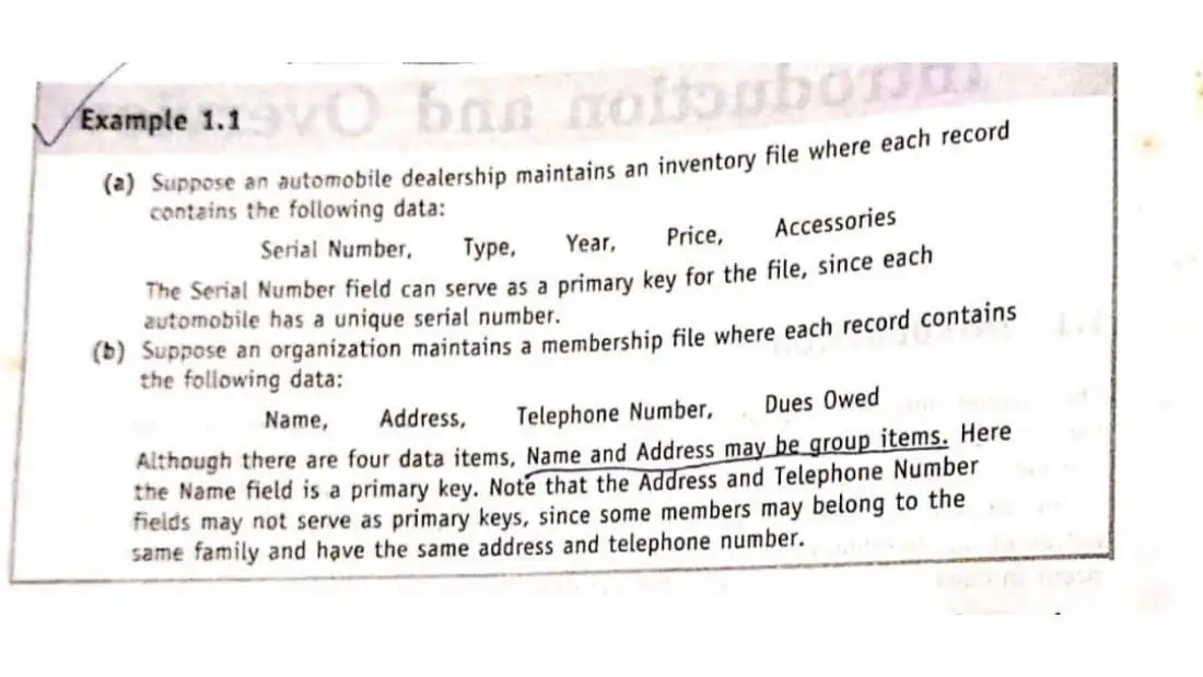
Each record in a file may contain many field items, but the value in a certain field may uniquely determine the record in the file. Such a field K is called primary key, and the values k1,k2,.. in such a field are called keys or key values.
Records may also be classified according to length.
A file can have fixed-length records or variable-length records
In fixed-length records, all the records contain the same data items with the same amount of space assigned to each data item.
In variable-length records, file records may contain different lengths.
For example, student records, usually have variable lengths, since different students take different numbers of courses.
The above organization of data into fields, records and files may not be complex enough to maintain and efficiently process certain collections of data.
For this reason, data are also organized into more complex type of structures. The study of such data structure, includes the following three steps:
-
Logical or mathematical description of the structure
-
Implementation of the structure on a computer
-
Quantitative analysis of the structure, which includes determining the amount of memory needed to store the structure and the time required to process the structure.
Data structures
- Data may be organized in many different ways; the logical or mathematical model of a particular organization of data is called a data structure.
- The choice of a particular data model depends on two consideration:
-
It must be rich enough in structure to mirror the actual relationships of the data in real world.
-
The structure should be simple enough that one can effectively process the data when necessary.
arrays
- The simplest type of data structure is a linear (one-dimensional) array.
- By a linear array, we mean a list of a finite number n of similar data elements referenced respectively by a set of n consecutive numbers, usually 1,2 ,3,....,n.
- If we choose the name A for the array, then the elements of A are denoted by subscript notation a1,a2,a3,...,an Or by the parentheses notation A(1), A(2), A(3),..., A(n)
Or by the bracket notation A[1],A[2], A[3],...,A[n]
Regardless of the notation, the number K in A[K] is
- called a subscript and A[K] is called a subscripted variable.
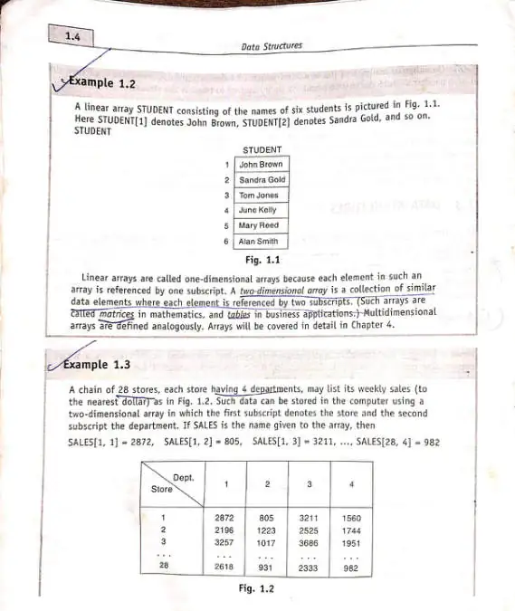
The size of the array is denoted by 28 X 4, since it contains 28 rows and 4 columns.
Linked lists
Suppose a brokerage firm maintains a file where record contains a customer’s name and his or her salesperson, and suppose the file contains the data appearing in the table shown below.
| Customer | Salesperson | |||
|---|---|---|---|---|
| 1 | Adams | Smith | ||
| 2 | Brown | Ray | ||
| 3 | Clark | Jones | ||
| 4 | Drew | Ray | ||
| 5 | Evans | Smith | ||
| 6 | Farmer | Jones | ||
| 7 | Geller | Ray | ||
| 8 | Hill | Smith | ||
| 9 | Infeld | Ray |
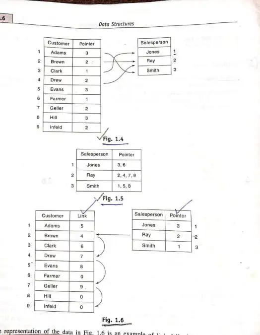
- Another way of storing the data above is to have a separated array for the salespeople and an entry (called a pointer) in the customer file which gives the location of each customer’s salesperson. Fig 1.4
- Fig 1.5 - Each salesperson have a set of pointers giving the positions of his or her customers.
- Fig 1.6 - Each sales person has one pointer which points to his or her first customer, whose pointer in turn points to the second customer, and so on, with the salesperson’s last customer indicate by 0. This is an example of linked list.
trees
Data often contain a hierarchical relationship between
- various elements. The data structure that reflects this relationship is called a rooted tree graph or simple a tree.
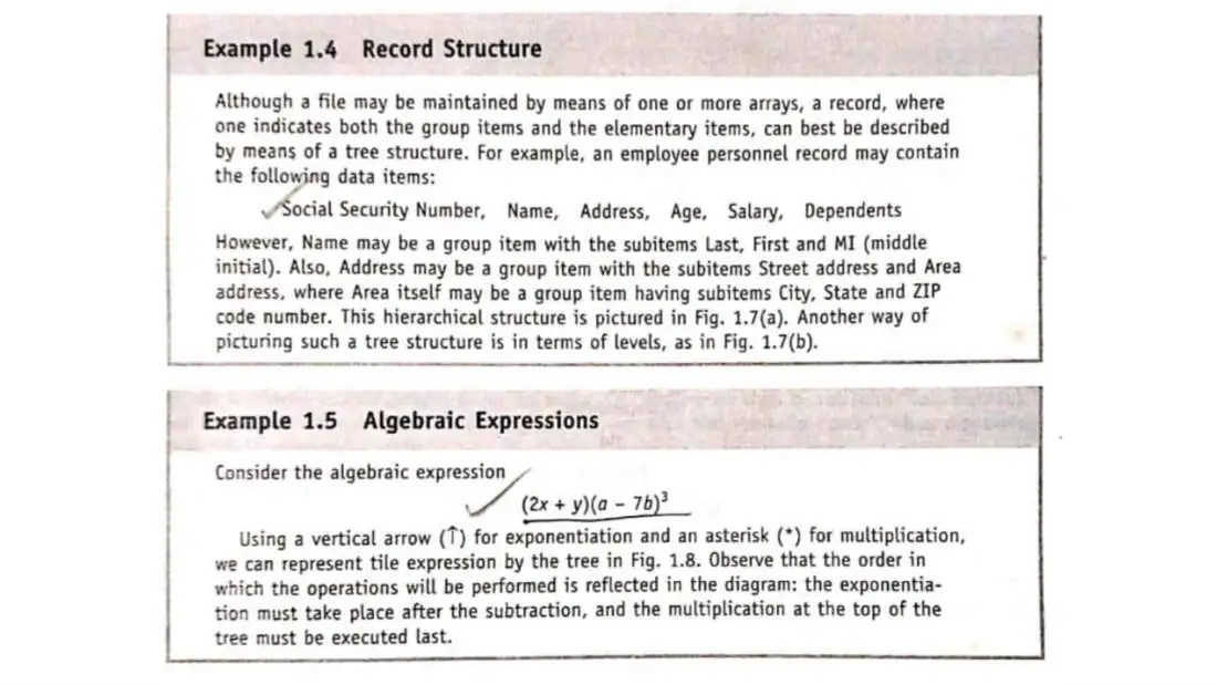
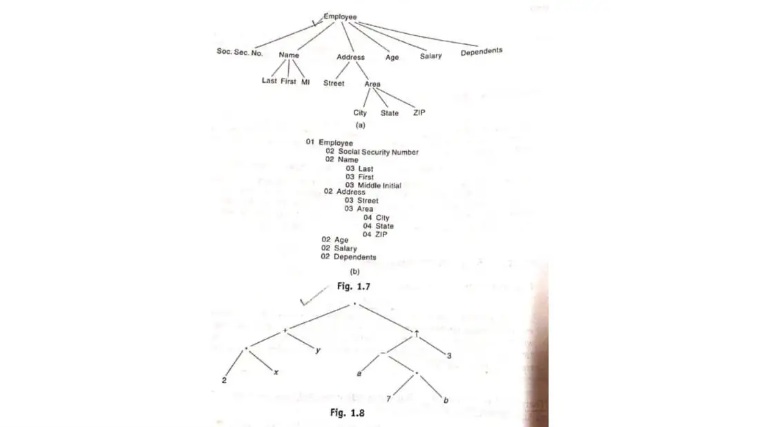
There are data structures other than arrays, linked list and trees. Some of these structures are briefly described below:
- Stack:
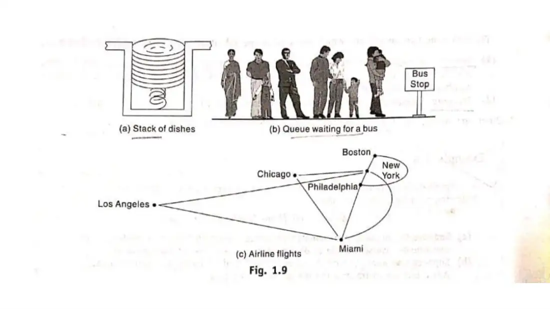
A stack also called a last-in first-out (LIFO) system, is a linear list in which insertions and deletions can take place only at one end, called the top. This structure is similar in its operation to a stack of dishes on a spring system as shown in the figure. Note that new dishes are inserted only at the top of the stack and dishes can be deleted only from the top of the stack
- Queue:
A queue, also called a first-in first-out (FIFO) system is a linear list in which deletions can take place only at one end of the list “the front” of the list, and insertions can take place only at the other end of the list, “the rear” of the list. This structure operates much the same way as a line of people waiting at a bus stop: the first person in the line is the first person to board the bus.
- Graph:
Data sometimes contain a relationship between pairs of elements which is not necessarily hierarchical in nature.
For example, suppose an airline flies only between cities connected by lines in the figure. The data structure which reflects this type of relationship is called a Graph.
Data structure operations
The data appearing in our data structure are processed by
- means of certain operation. In fact, the particular data structure that one chooses for a given situation depends largely on the frequency with which specific operations are performed.
The following four operations play a major role for this
- course:
- Traversing: Accessing each record exactly once so that certain items in the record may be processed. This accessing and processing is sometimes called “visiting” the record
Data structure operations
- Searching: Finding the location of the record with a given key value or finding the location of all records which satisfy one or more conditions
- Inserting: Adding a new record to the structure
- Deleting: Removing a record from the structure The following two operations, which are used in special situations :
- Sorting: Arranging the records in some logical order (e.g., alphabetically according to some NAME key, or in numerical order according to some NUMBER key, such as Social Security Number or account number)
- Merging: Combining the records in two different sorted files into a single sorted file.
Other operations like copying or concatenation will be discussed later.
Algorithms : complexity, time space tradeoff
An algorithm is a well-defined list of steps for solving
- a particular problem. One major purpose of this course, is to develop efficient algorithms for the processing of our data.
The time and space it uses are two major measures of the
- efficiency of an algorithm.
- The complexity of an algorithm is the function which gives the running time and/or space in terms of the input size.
Searching algorithms
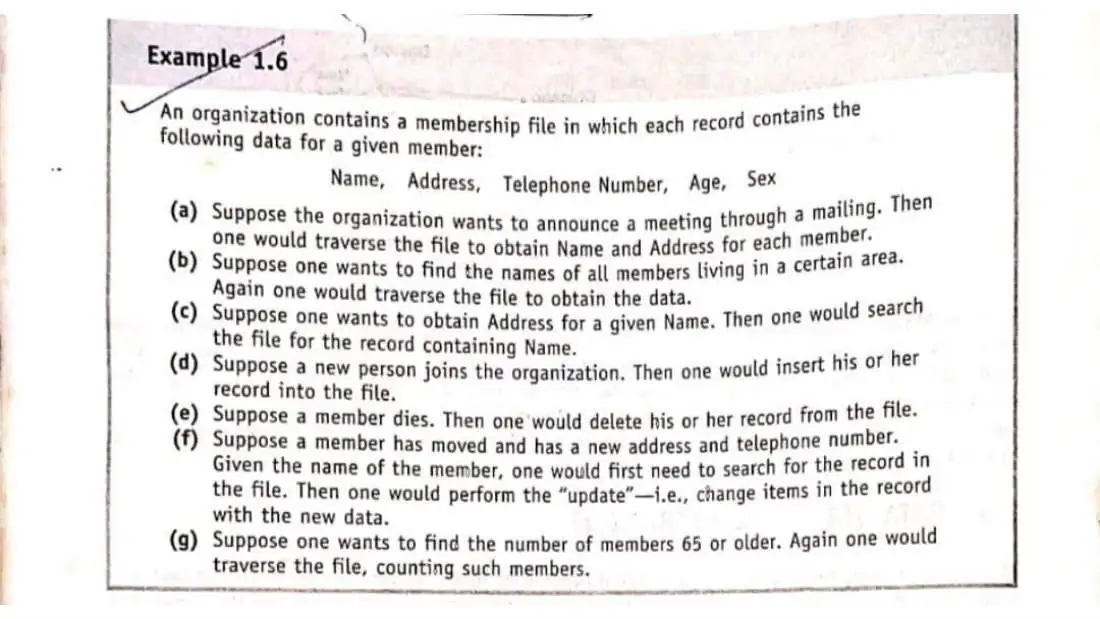
Consider a membership file, as in Example 1.6, in which each record contains, among other data the name and telephone number of its members. Suppose we are given the name of a member and we want to find his or her telephone number. One way to do is to linearly search through the file that is to apple the following algorithm.
Linear search
Search each record of the file one at a time, until finding the given Name and hence the corresponding Telephone Number.
- The time required to execute the algorithm is proportional to the number of comparisons. Also, assuming that each name in the file is equally likely to picked., it is intuitively clear that the average number of comparisons for a file with n records is equal to n/2 that is the complexity of the linear search algorithm is C(n) = n/2
- The above algorithm would be impossible in practice if we were searching through a list consisting of thousands of names, as in a telephone book..
Binary Search
- Compare the given name Name with the name in the middle of the list; this tells which half of the list contains Name.
Then compare Name with the name in the middle of the correct
- half to determine which quarter of the list contains Name.
- Continue this process until finding Name in the list
- The complexity of the binary search algorithm is given by:
C(n) = log n
- For example, one will not require more than 15 comparisons to find a given Name in a list containing 25000 names.
Although, the binary search algorithm is very efficient
- algorithm, it has some major drawbacks.
- Specifically, the algorithm assumes that one has direct access to the middle name in the list or a sublist. This means that the list must be stored in some type of array.
An example of time-space tradeoff
Suppose a file of records contains names, social security
- number and much additional information among its fields. Sorting the file alphabetically and usinga binary search
- is a very efficient way to find the record for a given name.
On the other hand, suppose we are given only the social
- security number of the person. Then we have to do linear search for the record, which is extremely time-consuming for a very large number of records.
Have another file which is sorted numerically according
- to social security number. This however, would double the space required for storing the data.
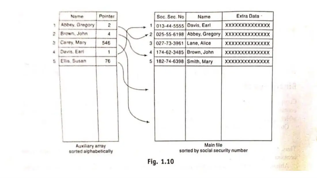
Another way, as shown in the figure, is to have the main
- file sorted numerically by social security number and to have an auxiliary array with only two columns, the first column containing an alphabetized list of the names and the second column containing pointers which give the locations of the corresponding records in the main file.
Exercises
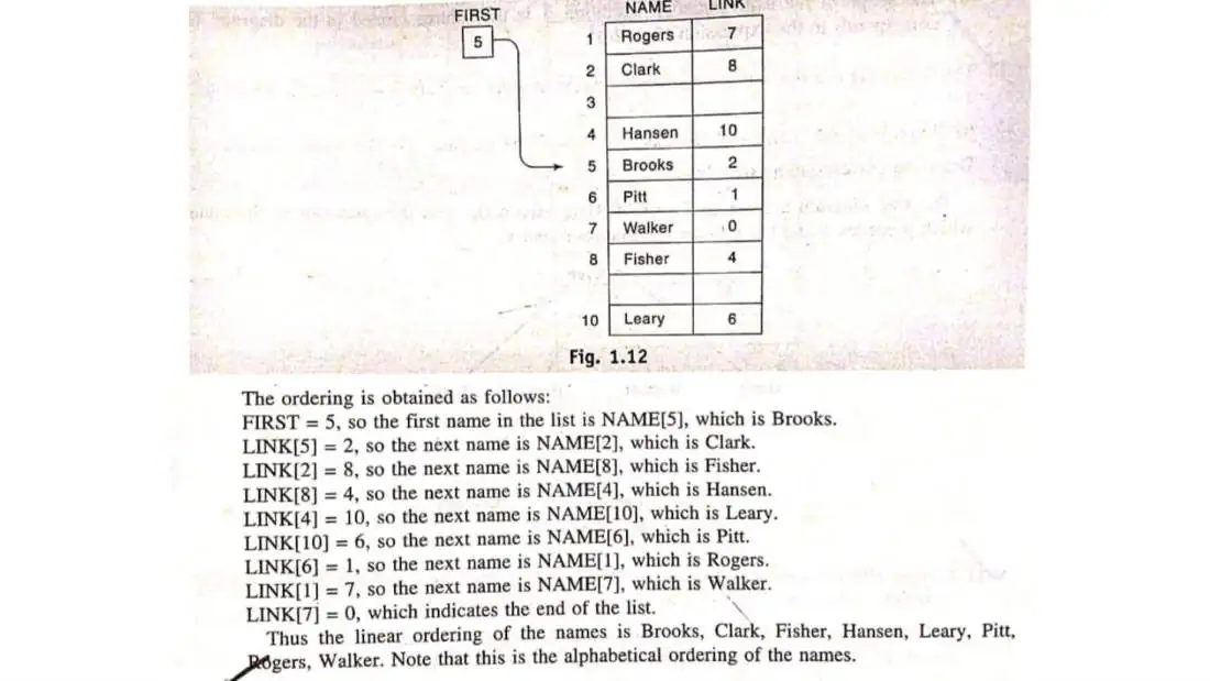
- Consider the linear array NAME in the figure. The values of FIRST and LINK[K] in the figure determines a linear ordering of the names as follows. FIRST gives the location of the first name in the list, and LINK[K] gives the location of the name following NAME[K], with 0 denoting the end of the list. Find the linear ordering of the names.
- Consider the algebraic expression (7x + y)(5a - b)3.
a.
Draw the corresponding tree diagram b.
Find the scope of the exponential operation (The scope of a node v in a tree is the subtree consisting of v and the nodes following v)
-
Discuss whether a stack or a queue is the appropriate structure for determining the order in which elements are processed in each of the following situations:
-
Batch computer programs are submitted to the computer center.
-
Program A calls subprogram B, which calls subprogram C, and so on.
-
Employees have a contract which calls for a seniority system for hiring and firing.
Answer
-
Queue. Excluding priority cases, programs are executed on a first come , first served basis
-
Stack. The last subprogram is executed first, and its results are transferred to the next-to-last program, which is then executed, and so on, until the original calling program is executed.
-
Stack. In a seniority system, the last to be hired is the first to be discharged.
-
Briefly describe the notions of (a) the complexity of an algorithm (b) the space-time tradeoff of algorithms.
Answer:
(a)
The complexity of an algorithm is a function f(n) which measures the time and/or space used by an algorithm in terms of the input size n.
(b)
The space-time tradeoff refers to a choice between algorithmic solutions of a data processing problem that allows one to decrease the running time of an algorithmic solution by increasing the space to store the data and vice versa.
- Suppose a data set S contains n elements.
a)
Compare the running time T1 of the linear search algorithm with the running time T2 of the binary search algorithm when (i) n = 1000 and (ii) n = 10,000 b)
Discuss searching for a given item in S when S is stored as a linked list
Answer:
a)
The expected running time of the linear search algorithm is f(n) = n/2 and that of the binary search is f(n) = log n.
i)
for n = 1000, T1 = 500 and T2 = 10 ii)
for = 10,000, T1 = 5000 and T2 = 14 b)
The binary search algorithm assumes that one can directly access the middle element in the set S. But one cannot directly access the middle element in a linked list. Hence one may have to use a linear search algorithm where S is stored as a linked list.
- The daily flights of an airline company appear in the following figure. CITY lists the cities and ORIG[K] and DEST[K] denote the cities of origin and destination, respectively, of the flight NUMBER[k]. Draw the corresponding directed graph of the data. (The graph is directed because the flight numbers represent flights from one city to another but not returning.
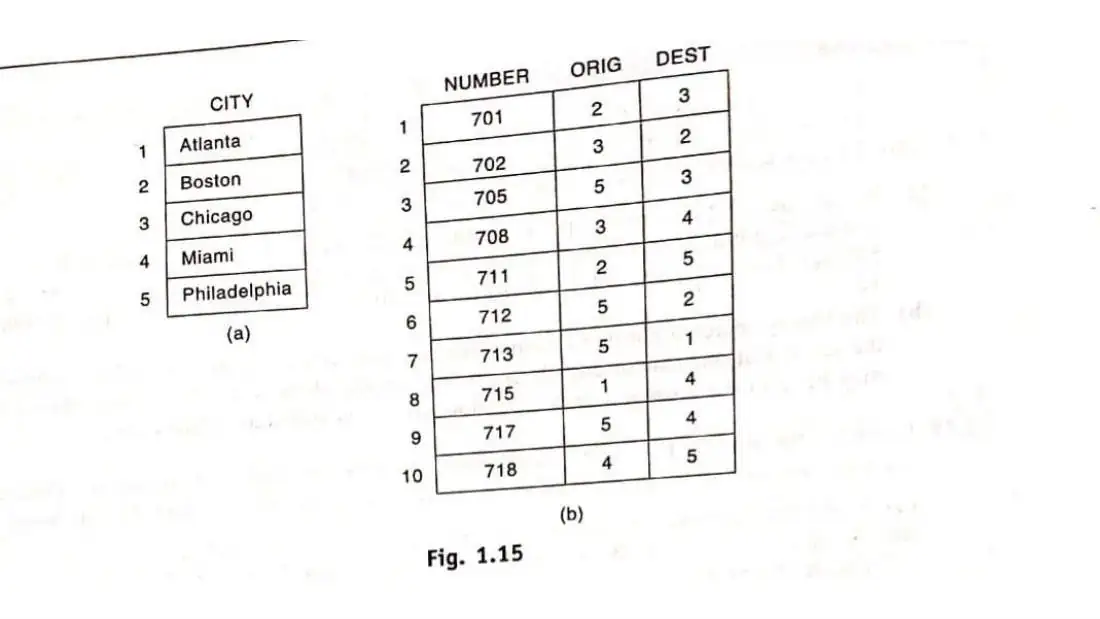
- Consider the data above, which gives the different flights of an airline. Discuss different ways of storing the data so as to decrease the time in executing the following:
a)
Find the origin and destination of a flight, given the flight number.
b)
Give city A and city B, find whether there is a flight from A to B, and if there is find its flight number.
Answer:
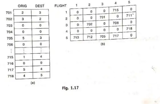
a) Store the data in arrays ORIG and DEST where the subscript is the flight number.
b) Store the data in a two-dimensional array FLIGHT where FLIGHT[J,K] contains the flight number of the flight from CITY[J] to CITY[K], or contains 0 when there is no such flight.
Mathematical notations and functions
The various mathematical functions which appear very often in the analysis of algorithms and in computer science, and their notations.
Remainder function; modular arithmetic
- The remainder function, commonly referred to in the context of modular arithmetic, plays a fundamental role in computer science, cryptography, algorithms, and number theory. Let's break it down clearly.
In mathematics and computer science, the remainder function refers to the
- operation that returns the remainder after one integer is divided by another.
- This is typically denoted using the modulo operator, written as:
a mod n
Example:
17 mod 5 = 2
Because 17 ÷ 5 = 3 with a remainder of 2.
Modular arithmetic is a system of arithmetic for integers where numbers "wrap around" upon reaching a certain value — the modulus.
Think of a clock: after 12 hours, it wraps back to 1. This is "mod 12" arithmetic.
14 mod 12 = 2 → 14 o’clock is 2 PM.
In general,
For integers a and n (with n > 0),
a mod n = r means that a = q × n + r, where:
q is the quotient (integer division),
- r is the remainder,
- and 0 ≤ r < n.
How is modular arithmetic used in computer science?
Modular arithmetic is everywhere in computer science. Here are key applications:
- Hashing and Hash Tables Used to map data of arbitrary size to fixed-size values. Example: If a hash table has 10 slots, use hash(key) mod 10 to determine which slot to store the data in.
Ensures the index stays within valid bounds.
- Cryptography Many encryption algorithms (like RSA, Diffie-Hellman) rely heavily on modular arithmetic.
Modular exponentiation: computing (a^b) mod n efficiently. Security relies on the difficulty of problems like modular discrete logarithms or factoring large numbers.
- Random Number Generation Pseudo-random number generators (PRNGs) often use modular operations.
Linear Congruential Generator (LCG):
X_{n+1} = (a × X_n + c) mod m
- Circular Buffers and Arrays
Used in data structures like queues or ring buffers.
Index calculation: (index + 1) mod buffer_size wraps around to 0 when reaching the end.
- Even/Odd, Parity, and Divisibility Checks
n mod 2 == 0 → even number
n mod 3 == 0 → divisible by 3
Used in algorithms to make decisions based on divisibility.
- Computer Arithmetic (Fixed-Size Integers)
Computers use modular arithmetic naturally due to fixed bit widths.
An 8-bit unsigned integer can represent 0 to 255.
Adding 1 to 255 gives 0 → this is addition modulo 256.
Important properties of modulo arithmetic
Let a, b, n be integers, and n > 0. Then:
-
(a + b) mod n = [(a mod n) + (b mod n)] mod n
-
(a − b) mod n = [(a mod n) − (b mod n)] mod n
-
(a × b) mod n = [(a mod n) × (b mod n)] mod n
-
a mod n = b mod n → a ≡ b (mod n) (congruence)
These allow efficient computation, especially with large numbers.
Handling Negative Numbers:
In programming, the behavior of modulo with negative numbers can vary. Mathematical definition: remainder should be non-negative.
Example: -7 mod 5 = 3 because -7 = (-2)×5 + 3 But in some languages (like Python), -7 % 5 gives 3, while in C/C++, it may give -2.
So, be cautious — always check how your programming language handles negative modulo.
summary
Concept Explanation
Modulo operation Returns the remainder of division: a mod n
Core Idea Numbers wrap around after reaching modulus n
Notation a mod n or a % n
Key Uses Hashing, Cryptography, Circular buffers
Critical insights Enables bounded, cyclic and secure computations
Exercise - 1
Compute the following modulo operations. Assume positive integers unless stated.
-
15 mod 4
-
100 mod 7
-
23 mod 5
-
0 mod 9
-
64 mod 8
Answer exercise-1
15 mod 4 = 3
100 mod 7 = 2 (7×14=98, 100−98=2)
23 mod 5 = 3
0 mod 9 = 0
64 mod 8 = 0
exercise-2
Use modular arithmetic properties to simplify and compute:
- (17 + 25) mod 6
→ Compute using: (a + b) mod n = [(a mod n) + (b mod n)] mod n
- (13 × 8) mod 5
→ Use: (a × b) mod n = [(a mod n) × (b mod n)] mod n
Answer Exercise-2
1.(17+25)=42 → 42 mod 6 = 0
Also: 17 mod 6 = 5, 25 mod 6 = 1, (5+1) mod 6 = 0
- 13 mod 5 = 3, 8 mod 5 = 3, 3×3=9 → 9 mod 5 = 4
Direct: 13×8=104 → 104 mod 5 = 4
Exercise-3
In a program, you want to trigger an action every 5th iteration in a loop from i = 1 to 30.
Write the condition using modulo to detect every 5th iteration.
Answer:
if i % 5 == 0: (triggers at i=5,10,15,...)
Exercise -4
A hash table has 13 slots. Given keys with hash values:
-
100 → which slot?
-
237 → which slot?
-
1000 → which slot?
(Use hash(key) mod 13)
Answer:
100 mod 13 = 9 (13×7=91, 100−91=9)
237 mod 13: 13×18=234 → 3 1000 mod 13: Try 13×76=988 → 12
exercise-5
You're implementing a circular buffer of size 8.
Current index = 7.
After adding 3 elements (incrementing index each time), what is the new index?
→ Use: (index + 1) mod 8 repeatedly.
Answer:
(7+1) mod 8 = 0, then 1, then 2 → After 3 steps: index = 2
exercise-6
An 8-bit register stores unsigned integers.
What is the result of 250 + 10 in this register?
(Hint: It wraps around using mod 256)
Answer:
250 + 10 = 260 → 260 mod 256 = 4
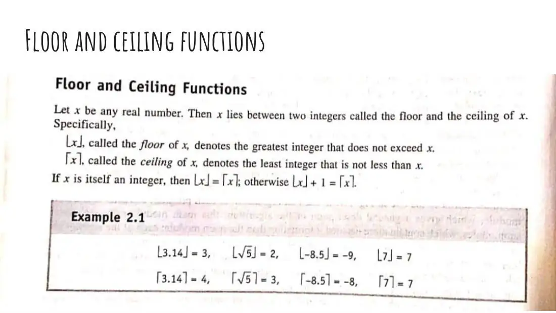
Integer and absolute value functions
- Integer functions deal with integers - whole numbers (positive, negative and
- Use in computer zero), without fractional parts. In science programming and computation, integers Array indexing: are often handled differently from
- real (floating-point) numbers due to converting efficiency and precision.
floating-point
- Common integer related functions results to valid
- Floor Function — ⌊x⌋ - The greatest indices.
integer less than or equal to x
- Algorithms Notation: floor(x) or ⌊x⌋ involving division and remainders. Examples:
- Binary search, tree ⌊3.7⌋ = 3 height ⌊-2.3⌋ = -3 calculations. ⌊5⌋ = 5
- Ceiling Function — ⌈x⌉ Use in CS:
- Memory allocation: rounding up to Definition: The smallest integer next whole block.
greater than or equal to x.
Pagination: number of pages =
- ⌈total_items / items_per_page⌉ Notation: ceil(x) or ⌈x⌉
- Network packet sizing.
Examples:
⌈3.2⌉ = 4 ⌈-1.7⌉ = -1 ⌈6⌉ = 6
- Truncate (or Truncation)
Use in CS:
- Type casting: (int)3.14 in C/C++ Definition: Remove the fractional truncated to 3.
part of a number — toward zero.
Fast conversion when rounding
- toward zero is acceptable. Examples:
trunc(4.9) = 4
trunc(-4.9) = -4
Difference from floor:
For negative numbers, trunc(-4.9) = -4, but floor(-4.9) = -5.
- Round Function Use in CS:
- User-facing output (e.g., display Definition: Round to the nearest numbers).
integer. Midpoints (like 2.5)
Converting sensor data or
- usually round to the nearest even floating-point results to integers. integer (banker’s rounding), though behavior varies.
Examples:
round(2.3) = 2
round(2.7) = 3
round(2.5) = 2 (in many systems)
Absolute Value Function — |x| or Examples: abs(x)
|5| = 5 Definition |-8| = 8 |0| = 0 Returns the magnitude (distance from zero) of a number, ignoring the sign.
Mathematical notation: |x| Function:
|x| = x if x ≥ 0 -x if x < 0
Applications of absolute function in computer science:
- Distance and error measurement
Compute distance between two points on a line: |a - b|
Measure error or deviation:
|predicted - actual| → absolute error
Applications of absolute function in computer science:
- Numerical Stability
Avoid negative values when only magnitude matters.
Prevent invalid inputs (e.g., negative array size).
Summary
| Function | Purpose | Example | CS use case |
|---|---|---|---|
| floor(x) | Greatest integer ≤ x | ⌊3.9⌋ = 3 | Array indexing |
| ceil(x) | Smallest integer ≥ x | ⌈3.1⌉ = 4 | Memory allocation |
| trunc(x) | Remove decimal part | trunc(-4.8) = -4 | Type casting |
| round(x) | Nearest integer | round(2.6) = 3 | Data display |
| abs(x) | Magnitude (no sign) | abs(-7) = 7 | Distance, error |
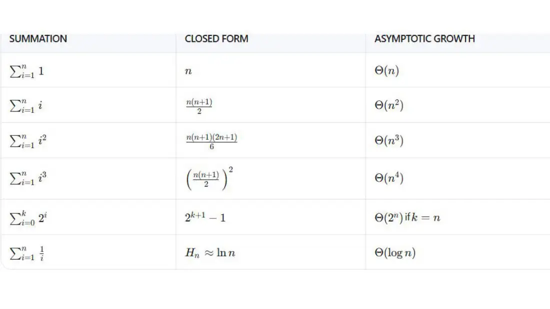
Summation symbols; sums
In algorithm analysis, we often
- need to compute how many times a statement runs — especially inside loops. Summation (denoted by the Greek letter sigma: ∑) lets us express and simplify these repeated operations.
It means add up f(i) for
- General Notation:
all integer values of i from a to b
Common summations and Closed formulas
- Sum of 1s (Constant sum):
It means you’re doing a constant operation n times.
Use case:
A simple loop that runs n times:
for(i = 0; i < n; i++{ print(“Hello there…”) }
Common summations and Closed formulas
- Sum of first n integers:
Use Case: Nested loops where inner loop grows with i. for (i = 0 i < n; i++{ for(j = 0 j <=i; j++{ print(i,j)
} }
Common summations and Closed formulas
- Sum of first n odd numbers:
Use Case: Algorithms that process odd indices or have quadratic behavior.
Common summations and Closed formulas
- Sum of squares:
Use Case: Triple nested loops or polynomial-time algorithms. for (i = 0;i<n;i++){ for(j = 0 ; j < i;j++){ for(k = 0; k <j;k++){ #some O(1) operations } } }
Common summations and Closed formulas
- Sum of cubes:
Less common, but appears in higher-order algorithms. Note: Sum of cubes = square of sum of integers.
Common summations and Closed formulas
- Arithmetic Series
General form of linear sequences.
Example: Loop with step size or offset.
Common summations and Closed formulas
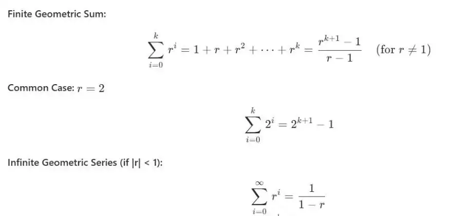
- Geometric Series
Use Case:
- Binary tree levels: number of nodes at each level is 2i
- Recursion trees: work per level decreases geometrically.
Common summations and Closed formulas
- Harmonic Series
Where γ is the Euler-Mascheroni constant (~0.5772).
Use Case:
- Average case of hash table insertion with chaining.
- Randomized algorithms like quicksort analysis.
Coupon collector problem: Expected time to collect all n coupons
- is
Factorial function
The factorial function is a fundamental mathematical
- concept widely used in computer science, combinatorics, probability, algorithm analysis, and recursion.
What is the factorial function?
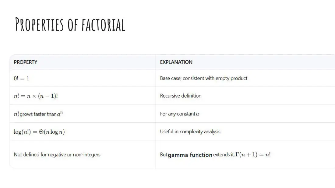
- The factorial of a non-negative integer n , denoted by n! , is the product of all positive integers less than or equal to n .

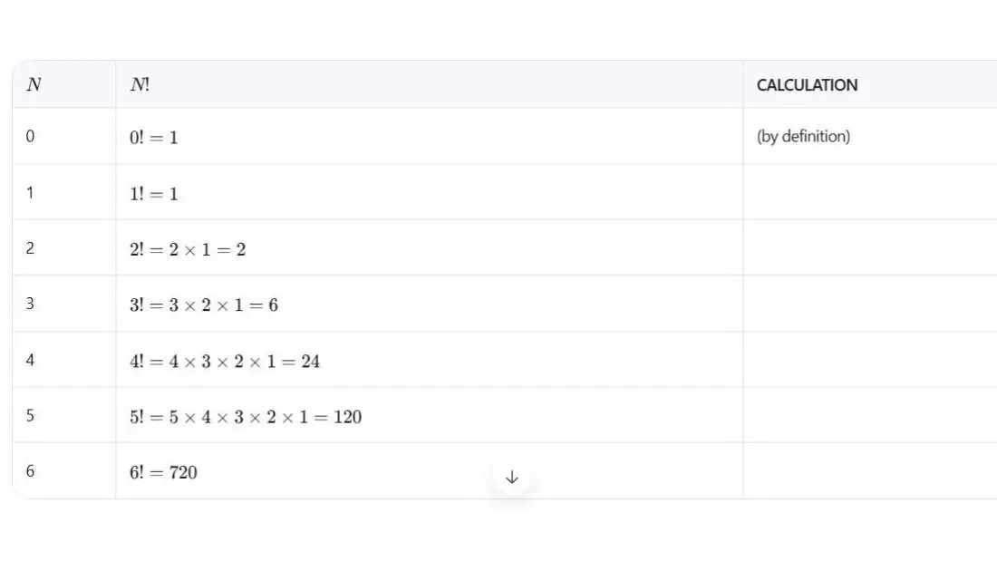
Recursive Definition:
The factorial function is a classic example of recursion:
Example:
4!=4×3!=4×3×2!=4×3×2×1!=4×3×2×1×0!=24
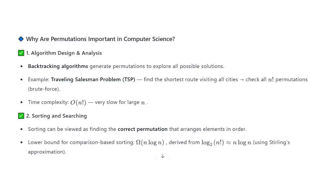
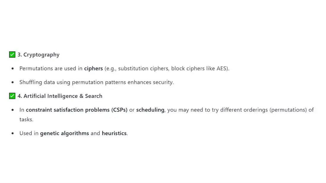
Where is factorial used in computer science?
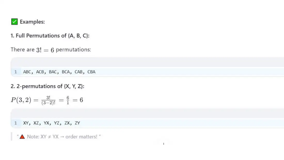
- Combinatorics & Permutations Number of ways to arrange n distinct items = n!
- Example: 3 books → 3!=6 possible orders.
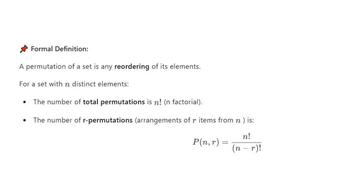
- Number of permutations of r items from n :
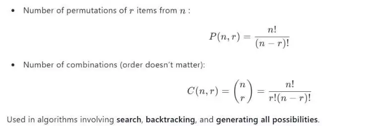
permutations
A permutation is an arrangement of all or part of a set of objects in a specific order.
Unlike combinations, order matters in permutations.
Exponents and logarithms
When analyzing algorithms, especially in computer science
- and data structures, we often need to describe how the runtime or space requirements of an algorithm grows as the input size increases.
Two mathematical concepts that are essential in this
- analysis are exponents and logarithms. They help us characterize the efficiency of algorithms and compare their performance using Big O notation.
Why exponents and logarithms matter?
Algorithms can have vastly different performance
- characteristics. Some run very quickly even on large inputs, while others become impractical as input size grows. Exponents and logarithms allow us to categorize these behaviors into meaningful growth rates:
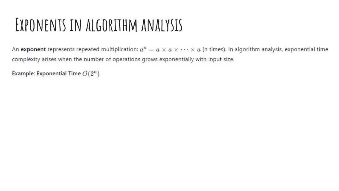
Consider a recursive algorithm to def fib(n):
if n <= 1:
compute Fibonacci numbers naively:
return n return fib(n-1) + fib(n-2)
This function makes two recursive calls for each input, leading to a call tree that doubles at each level. The number of calls grows like 2n, which is exponential.
Implication: Even for moderate values of n (e.g., n=50 ), the algorithm becomes extremely slow.
Use Case: Exponential algorithms are typically only feasible for very small inputs.
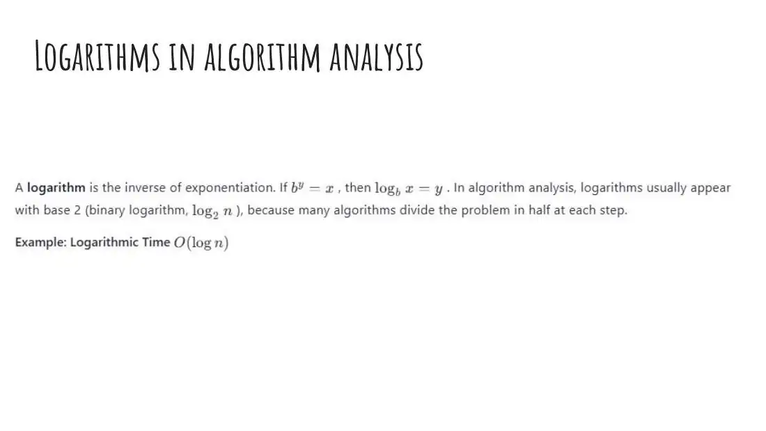
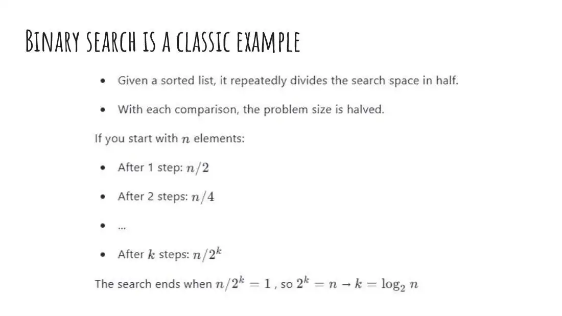
Time complexity: O(log n)
Implication: Even for very large n (e.g. 1 billion), log (109) = 30 steps suffice.
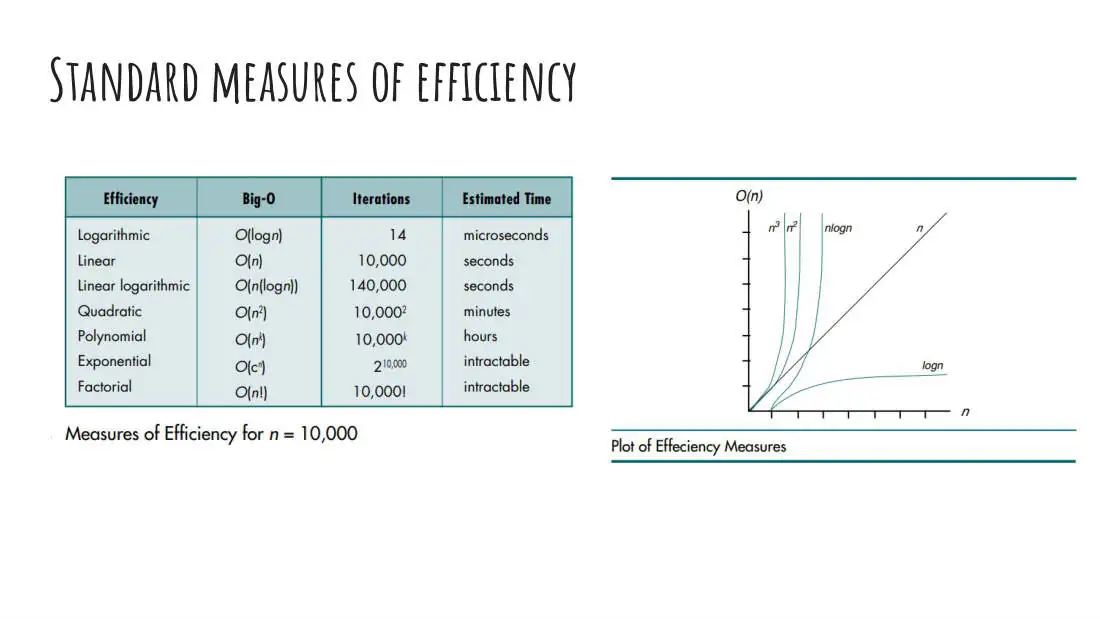
Common growth rates (Ordered by efficiency)
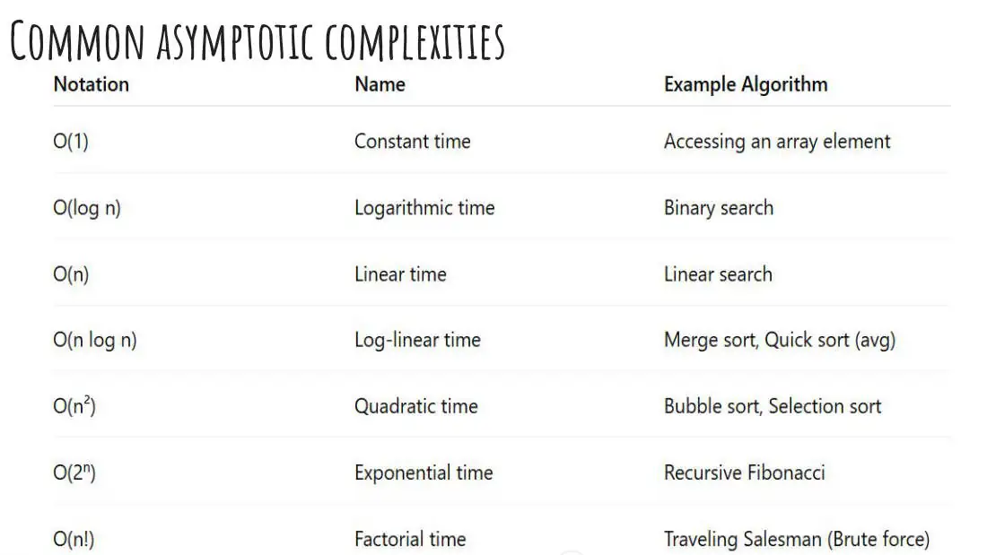
| Complexity | Name | Example Algorithms | ||
|---|---|---|---|---|
| O(1) | Constant | Accessing array element | ||
| O(log n) | Logarithmic | Binary Search | ||
| O(n) | Linear | Linear Search | ||
| O(n log n) | Linearithmic | Merge Sort, Quick Sort (average) | ||
| O(n2) | Quadratic | Bubble sort | ||
| O(2n) | Exponential | Naive Fibonacci, subset generation | ||
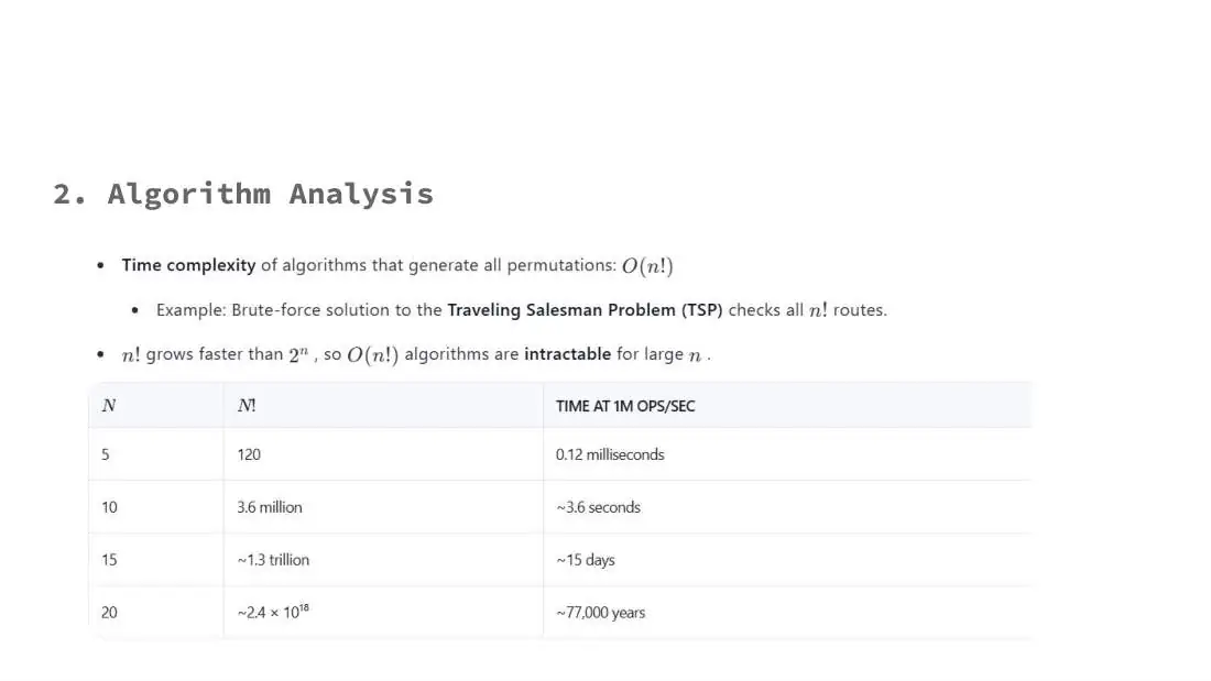
| O(n!) | O(n!) | Factorial | Traveling Salesman (brute force) |
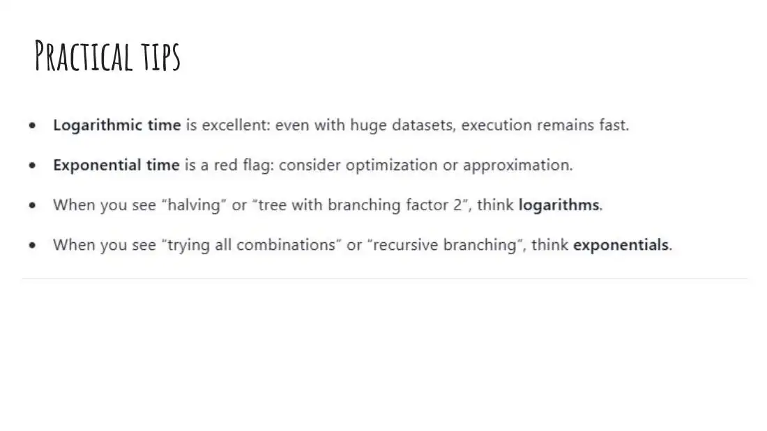
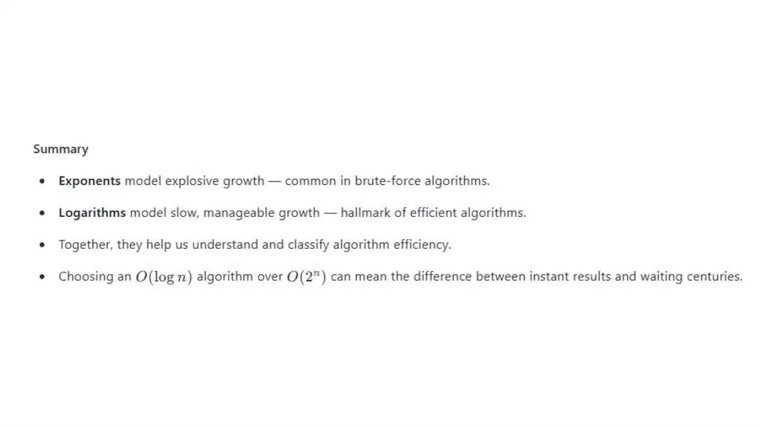
Logarithmic and Linearithmic algorithm scale well; exponential ones do not
Algorithmic notation
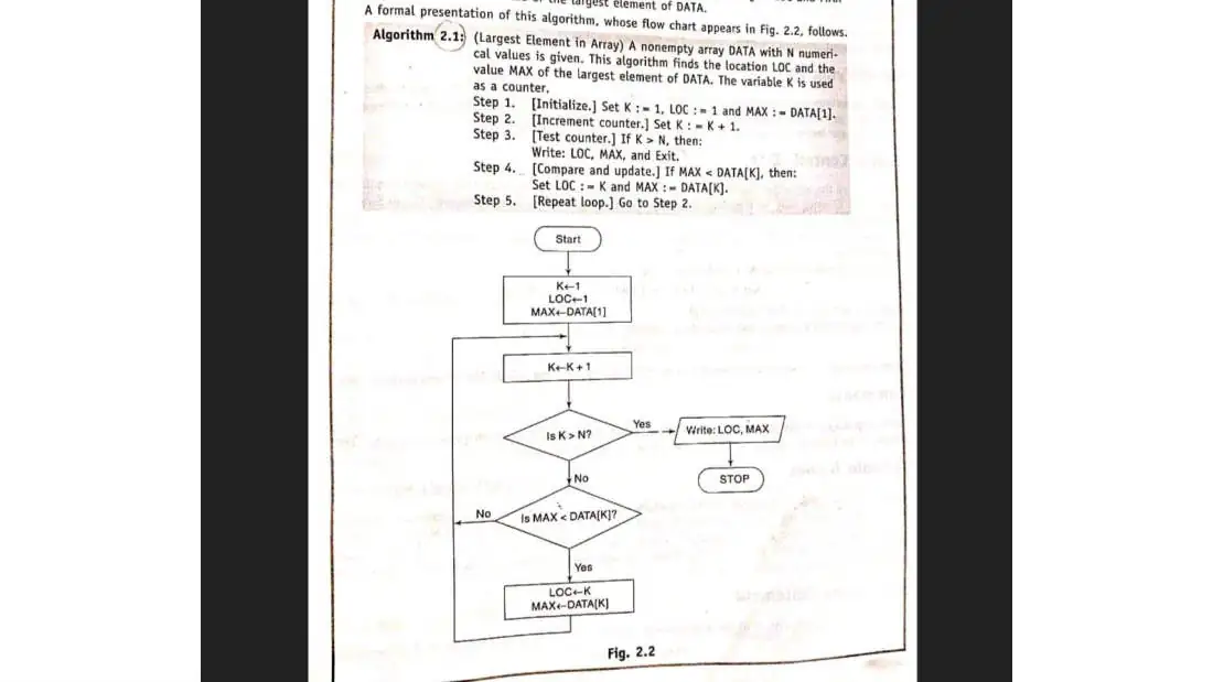
-
Identifying Number
-
Steps, Control, Exit
-
Comments
-
Variable Names
-
Assignment Statement
-
Input and Output
-
Procedures
Control structures
-
Sequence logic or sequential flow
-
Selectic logic or conditional flow
-
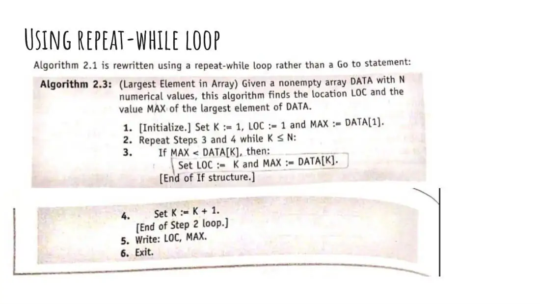
Iteration logic or repetitive flow
Asymptotic notation
When analyzing algorithms, we want to:
- Compare their efficiency, especially in terms of time and space.
Ignore machine-dependent constants and lower-order
- terms.
- Focus on input size (n) and how it affects performance as n grows large.
This leads to Asymptotic Analysis, which examines the behavior of algorithms as input size → ∞.
Basic terminologies
Term Description
Input Size(n)
The size of the input data (e.g., number of elements in an array)
Time complexity Number of basic operations or steps algorithm takes
Space Complexity Amount of extra memory used by the algorithm
What is asymptotic notation?
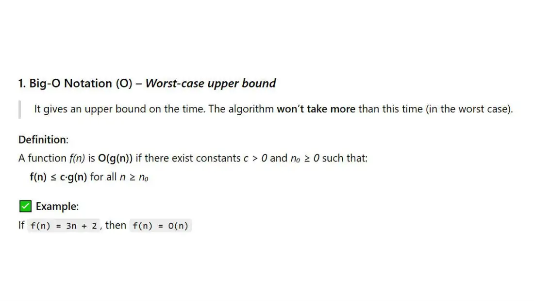
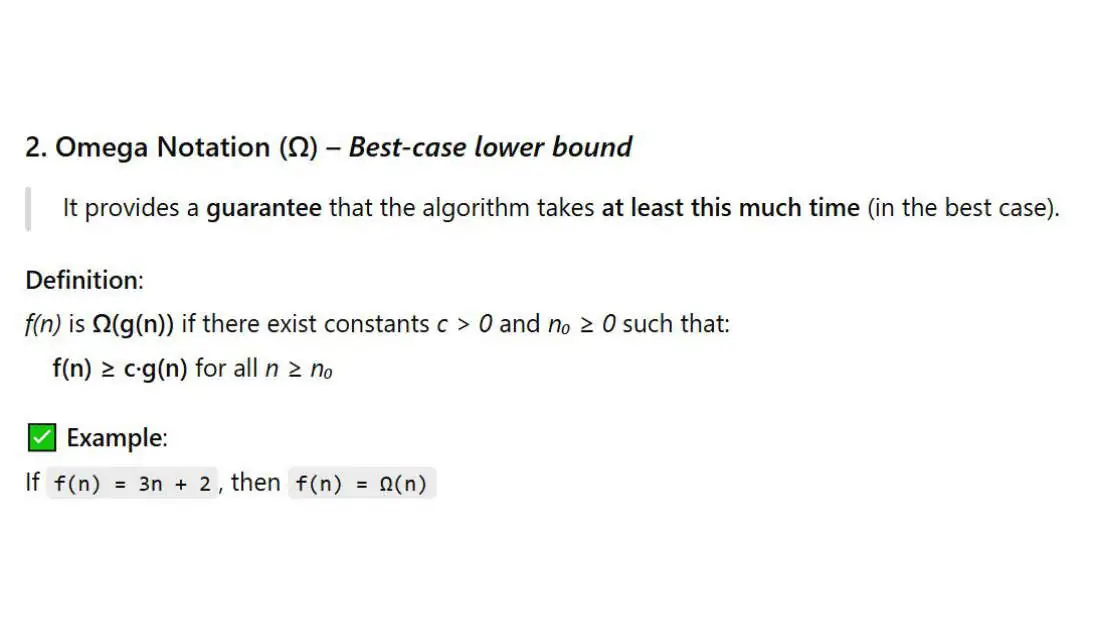
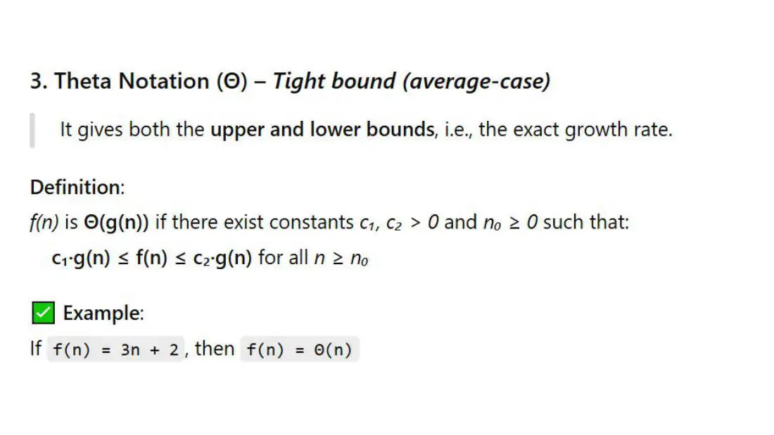
Asymptotic notation provides a mathematical way to describe the upper, lower, and tight bounds of an algorithm’s complexity.
There are 3 primary notations:
-
Big-O notation - worst-case upper bound
-
Big-Omega notation - best-case lower bound
-
Theta notation - tight-bound average case
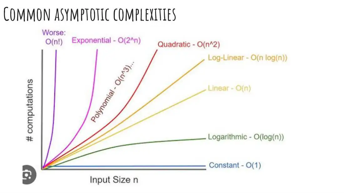
- An algorithm is said to have constant time with order O (1) when it is not dependent on the input size n. Irrespective of the input size n, the runtime will always be the same.
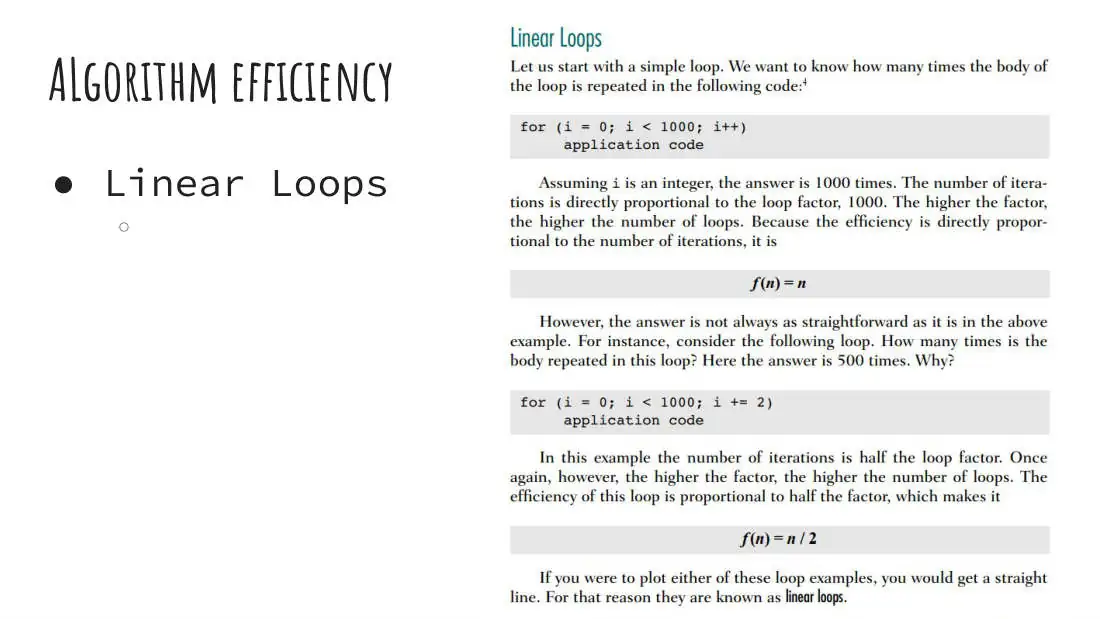
- An algorithm is said to have a linear time complexity when the running time increases linearly with the length of the input. When the function involves checking all the values in input data, with this order O(n).
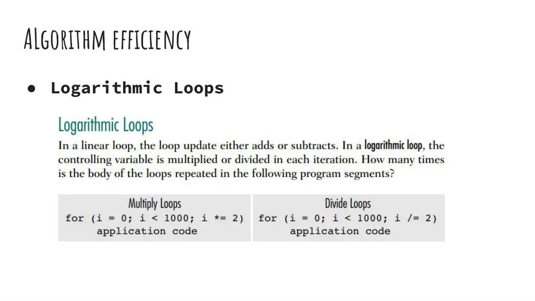
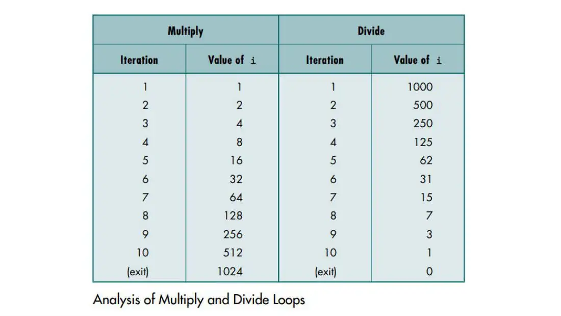
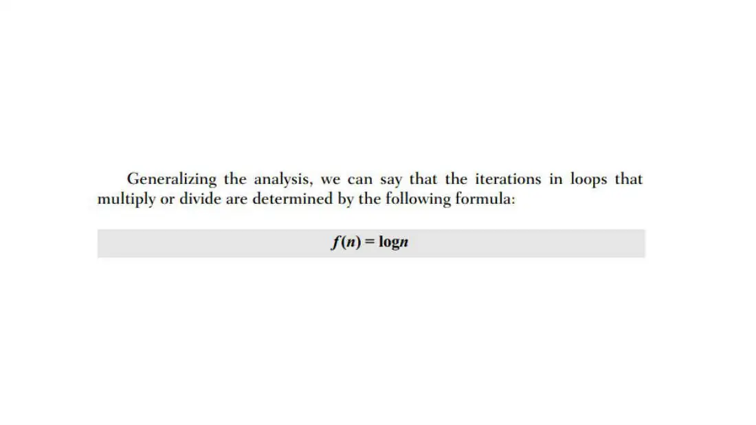
- An algorithm is said to have a logarithmic time complexity when it reduces the size of the input data in each step.
This indicates that the number of operations is not
- the same as the input size. The number of operations gets reduced as the input size increases.
- Algorithms are found in binary trees or binary search functions. This involves the search of a given value in an array by splitting the array into two and starting searching in one split. This ensures the operation is not done on every element of the data.
- An algorithm is said to have a non-linear time complexity where the running time increases non-linearly (n^2) with the length of the input.
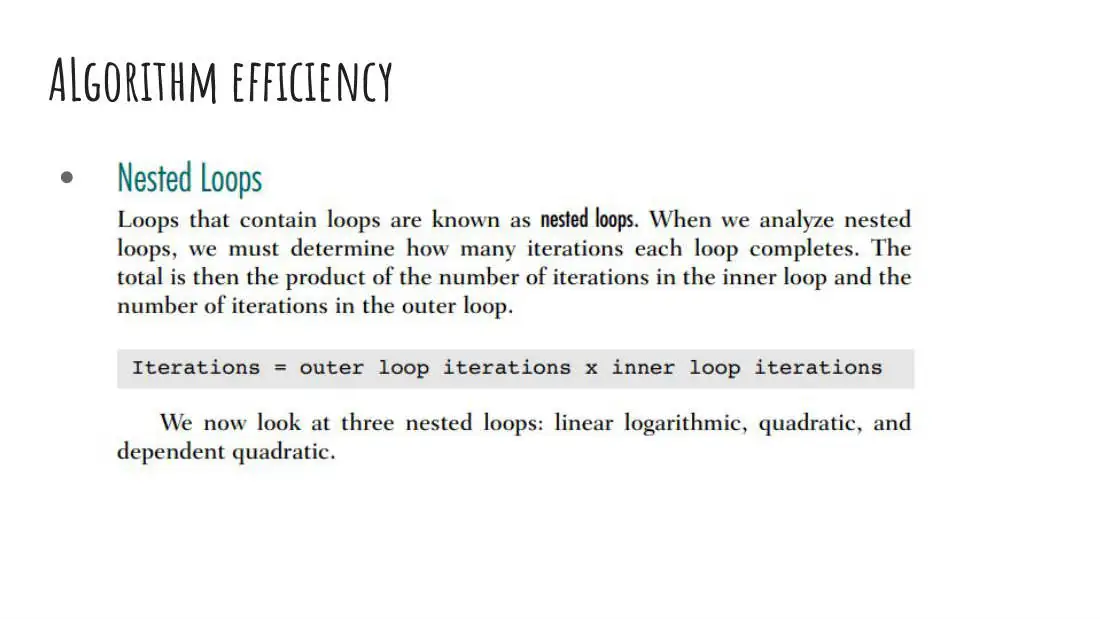
- Generally, nested loops come under this order where one loop takes O(n) and if the function involves a loop within a loop, then it goes for O(n)*O(n) = O(n^2) order.
- Similarly, if there are ‘m’ loops defined in the
- function, then the order is given by O (n ^ m), which are called polynomial time complexity functions.
How to compute big-o from a given problem or code
Step 1: Identify the Input Size (n)
Figure out what n represents. Common examples:
- Length of an array
- Number of elements in a list
- Number of nodes in a tree
- Size of a string
How to compute big-o from a given problem or code
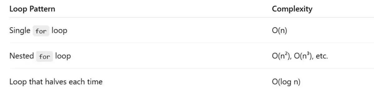
Step 2: Look for Loops
Every loop often contributes to the complexity.
How to compute big-o from a given problem or code
Step 3: Count nested for i in range(n): # O(n)
for j in range(n): # O(n)
structures print(i, j) # Total: O(n × n) = O(n²)
If you see one loop inside another, multiply their complexities:
How to compute big-o from a given problem or code
Step 4: Analyze Recursion (if present)
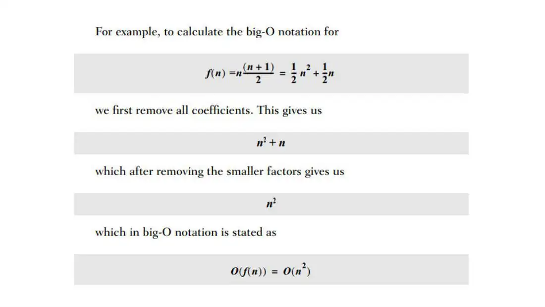
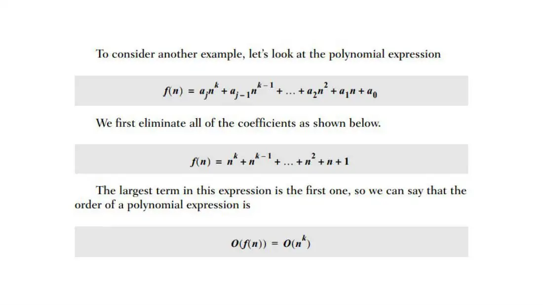
Use recurrence relations or recursion trees to compute time. Step 5: Ignore Constants and Lower Order Terms
- Drop constants:
O(2n) → O(n)
O(100n + 50) → O(n)
Drop lower-order terms:
- O(n² + n) → O(n²)
How to compute big-o from a given problem or code
Step 6: Add or Multiply Based on Control Flow
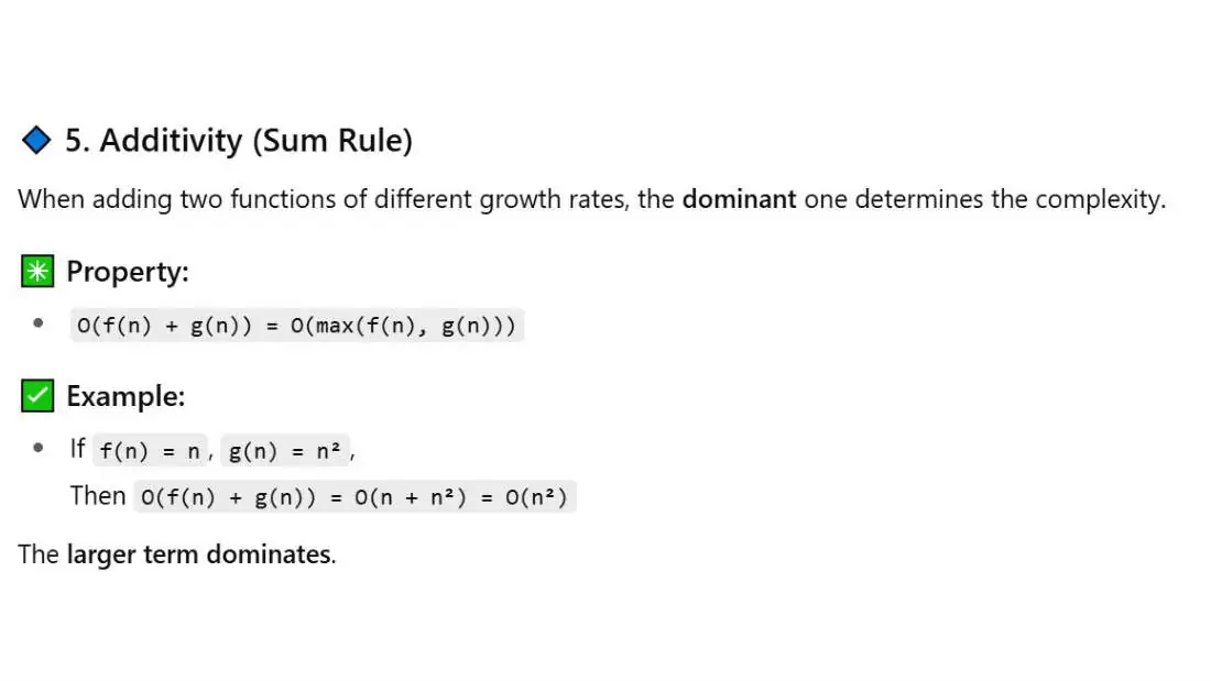
Sequential operations → Add complexities
O(n) + O(log n) = O(n)
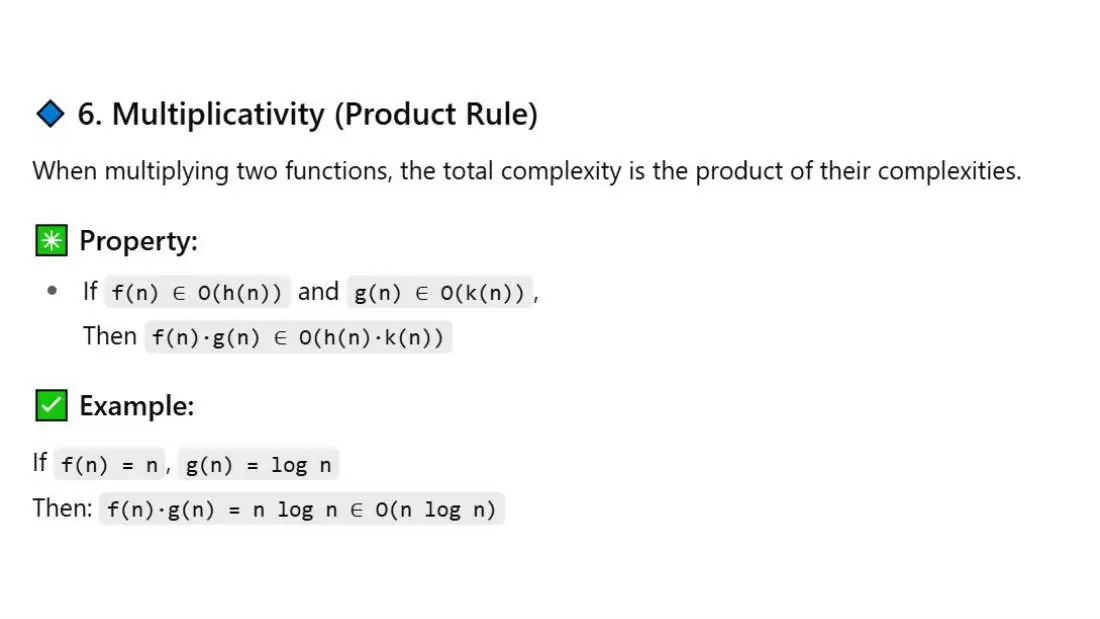
Nested operations → Multiply complexities
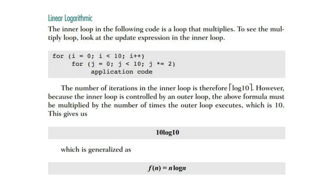
O(n) * O(log n) = O(n log n)
How to compute big-o from a given problem or code
Step 7: Use Big-O rules
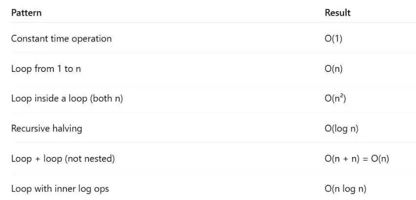
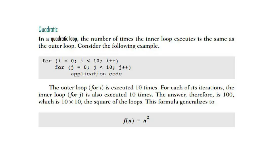
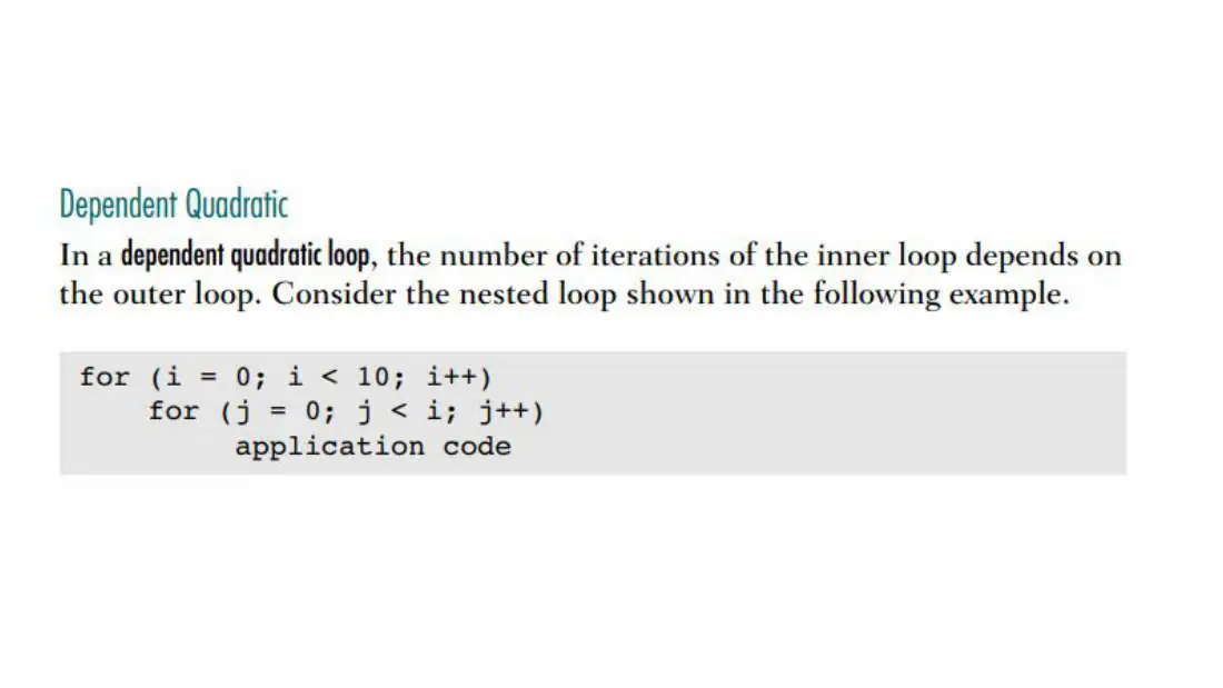
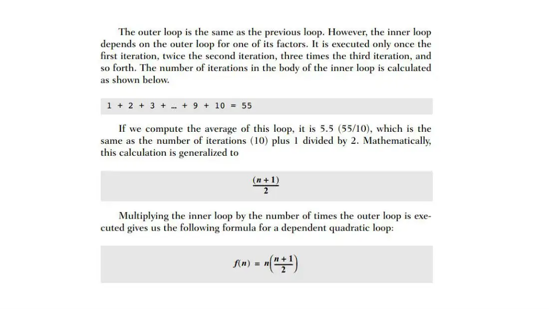
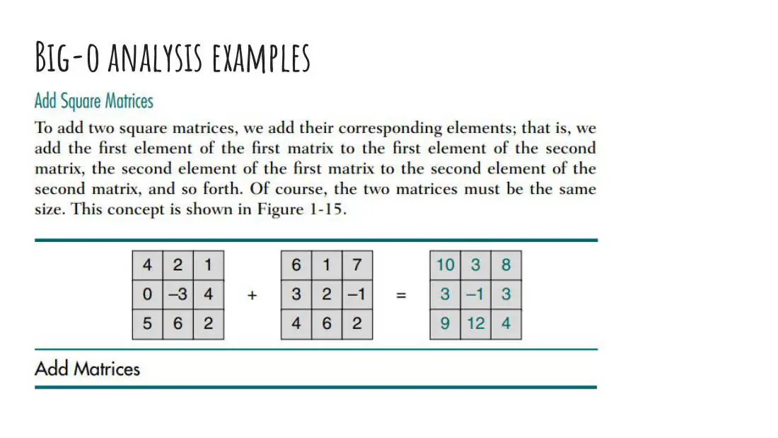
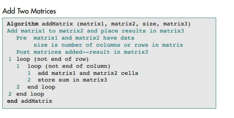
In this algorithm, we see that for each element in a row, we add all of the elements in a column. This is the classic quadratic loop. The efficiency of the algorithm is O(n2)
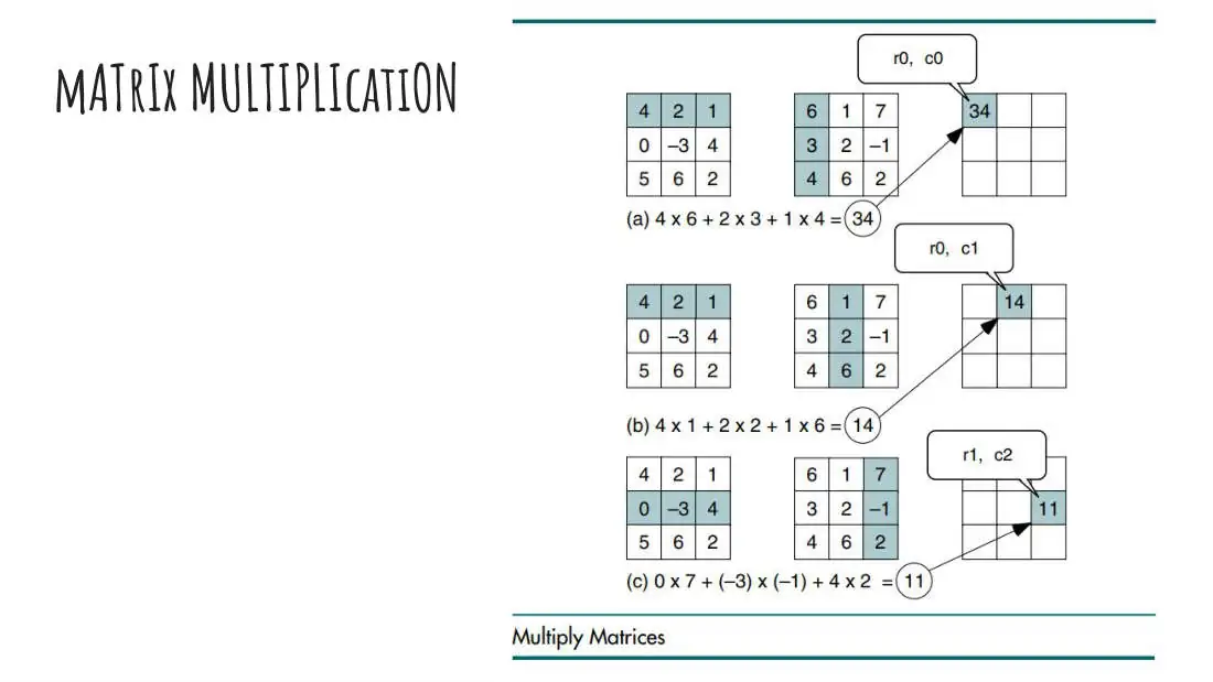
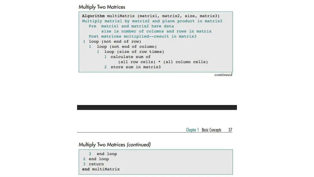
In this algorithm we see three nested loops. Because each loop starts at the first element, we have a cubic loop. Loops with three nested loops have a big-O efficiency of O(n3)
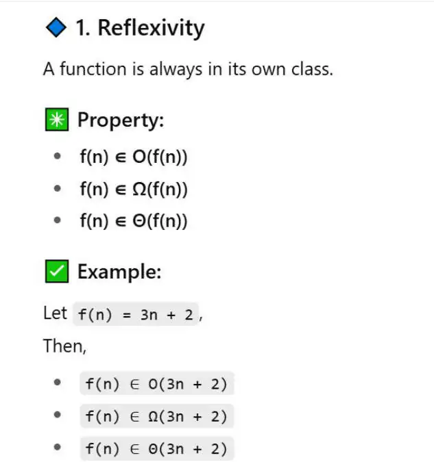
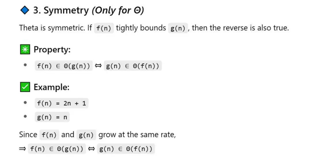
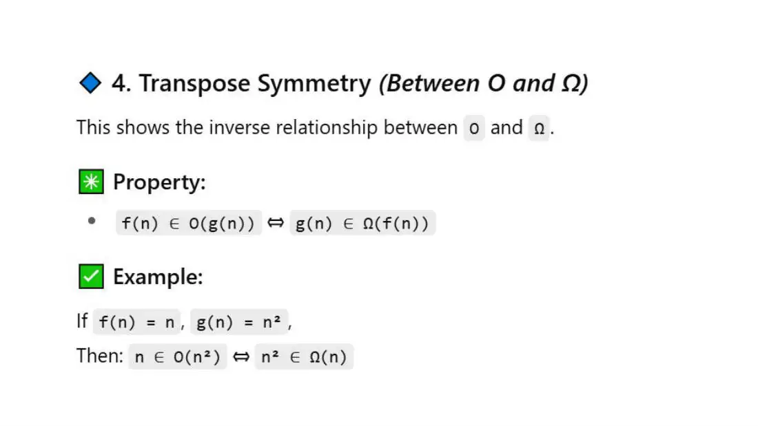
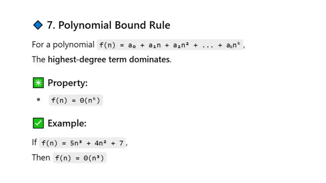
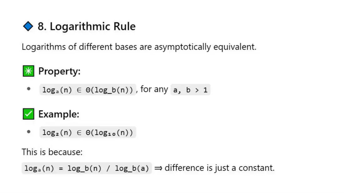
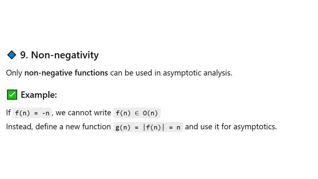
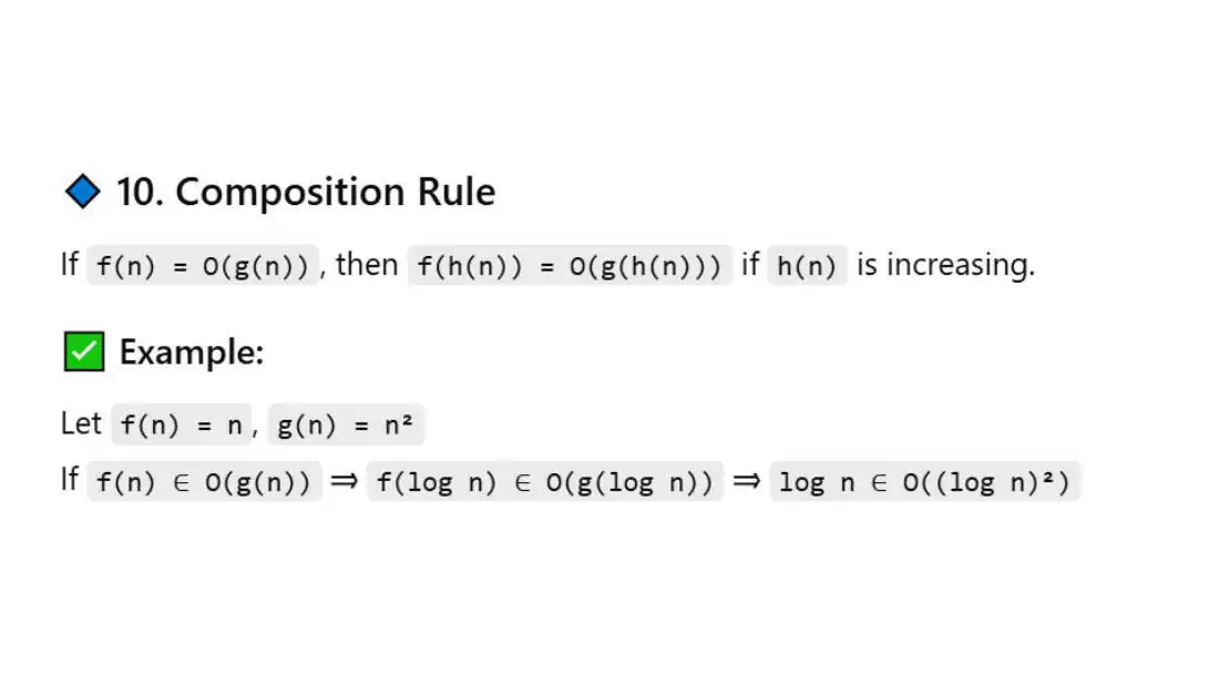
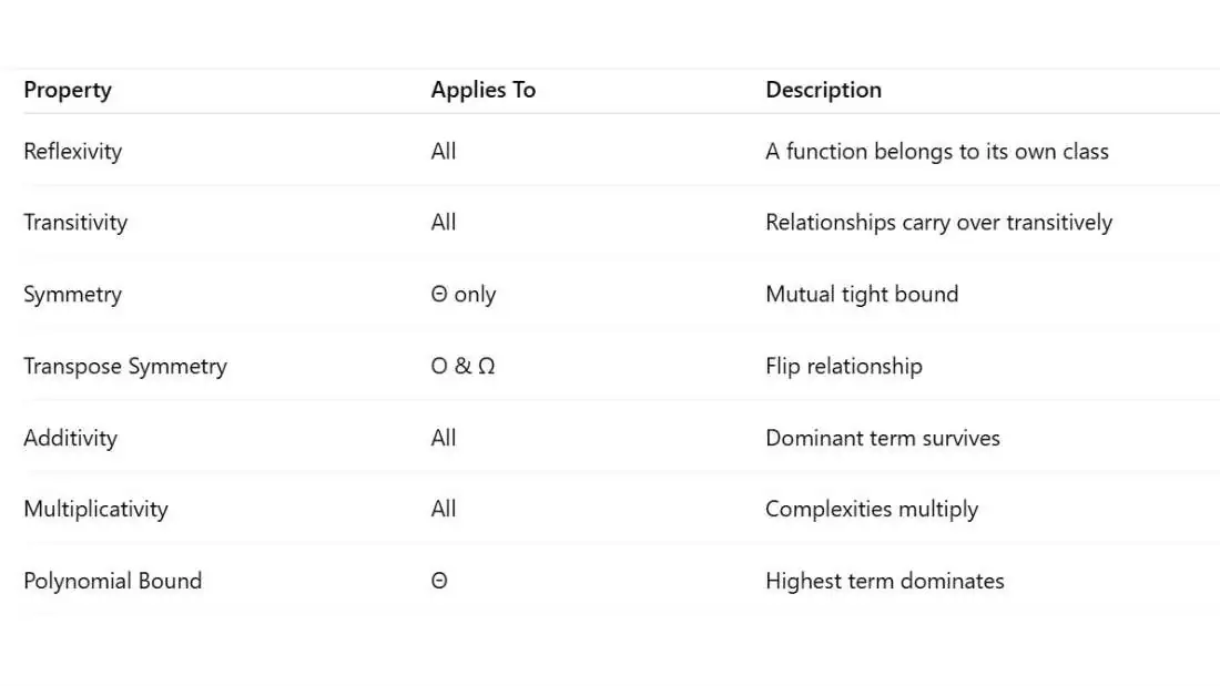
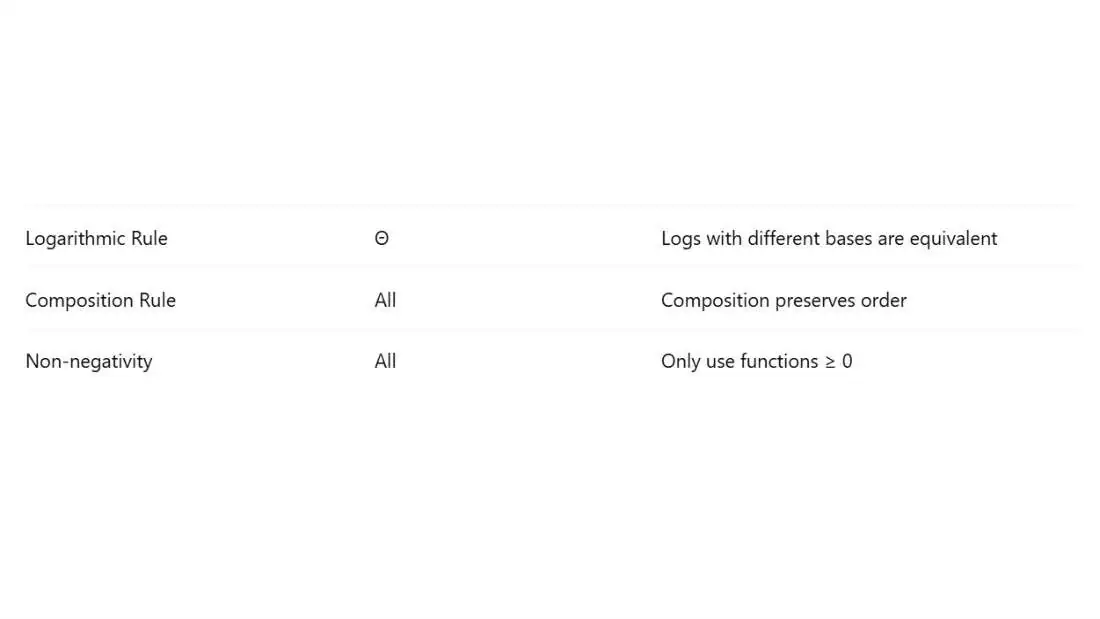
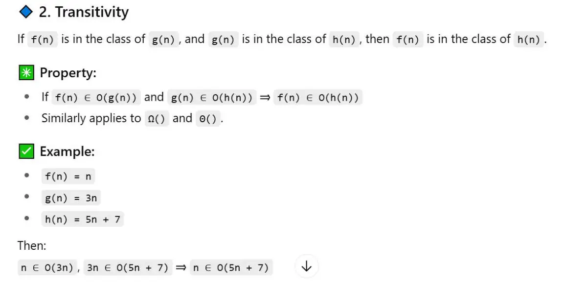
Common Properties of
asymptotic notations
Common Properties of asymptotic notations
Common Properties of asymptotic notations