Asymptotic Notation
Analyzing the Efficiency and Growth of Algorithms
Lecture Notes for Second Year Undergraduate Students (B.E./B.Tech — Computer Science / IT)
"Asymptotic notation describes the limiting behavior of an algorithm's running time as the input size grows toward infinity, allowing us to compare algorithms independently of hardware, compiler, or programming language."
Figure 0: Growth rates of common time complexities — the single most important picture in this course.
1. Introduction and Motivation
Suppose two students write two different programs to sort the same list of numbers. Both programs produce the correct sorted output. How do we decide which program is “better”? Running both on a laptop and comparing stopwatch times is unreliable — the result depends on the machine's speed, the programming language, background processes, compiler optimizations, and the specific input used.
What we actually want to know is: how does the amount of work grow as the input size n grows? This question is answered by analyzing an algorithm's time complexity (and space complexity) as a mathematical function of n, and then classifying that function using Asymptotic Notation — a set of mathematical tools (Big-O, Big-Omega, Big-Theta, little-o, little-omega) that describe the rate of growth of a function while ignoring machine-dependent constants and lower-order terms.
1.1 Learning Objectives
- Explain why asymptotic analysis is used instead of direct time measurement to compare algorithms.
- State the formal mathematical definitions of Big-O, Big-Omega, and Big-Theta notation.
- Prove or disprove simple asymptotic bound claims using the formal definitions.
- Apply standard rules (sum rule, product rule, dropping constants/lower-order terms) to derive the time complexity of code fragments.
- Analyze loops, nested loops, and simple recursive algorithms for their time complexity.
- Relate asymptotic notation to real algorithm case studies (searching, sorting) and real-world CS applications.
2. Why Not Just Measure Running Time Directly?
Direct timing (using a stopwatch or a profiler) is affected by many factors that have nothing to do with the algorithm's inherent efficiency:
| Factor | Problem |
|---|---|
| Hardware | A faster CPU/more RAM makes any algorithm look better, without the algorithm itself being any smarter. |
| Programming Language / Compiler | A C implementation of an O(n²) algorithm may run faster in absolute seconds than a Python implementation of an O(n log n) algorithm for small n, which is misleading for large-scale conclusions. |
| Input Instance | The same algorithm can run fast on one input and slow on another of the same size (e.g., Quicksort on an already-sorted array vs. a random array). |
| System Load | Background processes, cache states, and operating-system scheduling introduce noise/variability into wall-clock measurements. |
Asymptotic notation solves this by abstracting away constant factors and machine-specific details, focusing purely on how the number of basic operations scales as the input size n becomes large. This makes analysis portable: the conclusion “Merge Sort is O(n log n)” holds true regardless of which machine, language, or compiler is used.
3. Big-O Notation — The Upper Bound
Big-O notation describes an upper bound on the growth rate of a function. Informally, f(n) = O(g(n)) means “f(n) does not grow faster than g(n), for large enough n.” It is the most commonly used notation because it gives us a guarantee on the worst-case behavior of an algorithm — a promise that the algorithm will never be slower than a certain rate of growth.
3.1 Formal Definition f(n) = O(g(n)) if and only if there exist positive constants c and n₀ such that:0 ≤ f(n) ≤ c · g(n) for all n ≥ n₀
In words: beyond some threshold input size n₀, the function f(n) is always bounded above by some constant multiple c of g(n).
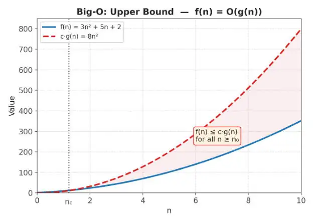
Figure 1: f(n) = 3n² + 5n + 2 stays below c·g(n) = 8n² for every n ≥ n₀, so f(n) = O(n²).
3.2 Worked Example
Claim: 3n² + 5n + 2 = O(n²)
Proof: We need to find constants c and n₀ such that 3n² + 5n + 2 ≤ c·n² for all n ≥ n₀.
- For n ≥ 1: 5n ≤ 5n² and 2 ≤ 2n²
- So 3n² + 5n + 2 ≤ 3n² + 5n² + 2n² = 10n²
- Choosing c = 10 and n₀ = 1 satisfies the definition. Hence 3n² + 5n + 2 = O(n²). ■ Note: We could also have proven O(n³) or O(2ⁿ) using the same technique — Big-O only requires that the bound hold, not that it be the tightest possible bound. In practice, we always report the tightest (smallest) g(n) that works, since that is the most informative statement.
4. Big-Omega Notation — The Lower Bound
Big-Omega notation describes a lower bound on the growth rate of a function. Informally, f(n) = Ω(g(n)) means “f(n) grows at least as fast as g(n), for large enough n.” It is used to express a guarantee about the best case or an inherent minimum amount of work a problem requires (e.g., any comparison-based sorting algorithm requires Ω(n log n) comparisons in the worst case).
4.1 Formal Definition f(n) = Ω(g(n)) if and only if there exist positive constants c and n₀ such that:0 ≤ c · g(n) ≤ f(n) for all n ≥ n₀
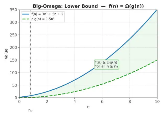
Figure 2: f(n) = 3n² + 5n + 2 stays above c·g(n) = 1.5n² for every n ≥ n₀, so f(n) = Ω(n²).
4.2 Worked Example Claim: 3n² + 5n + 2 = Ω(n²)
Proof: We need constants c and n₀ such that c·n² ≤ 3n² + 5n + 2 for all n ≥ n₀.
- For all n ≥ 1: 3n² + 5n + 2 ≥ 3n² (since 5n + 2 ≥ 0)
- Choosing c = 3 and n₀ = 1 satisfies the definition. Hence 3n² + 5n + 2 = Ω(n²). ■
5. Big-Theta Notation — The Tight Bound
Big-Theta notation describes a tight bound — a function that is bounded both above and below by the same rate of growth. f(n) = Θ(g(n)) means f(n) grows at exactly the same rate as g(n), up to constant factors. This is the strongest and most precise of the three main notations.
5.1 Formal Definition f(n) = Θ(g(n)) if and only if there exist positive constants c₁, c₂, and n₀ such that:c₁ · g(n) ≤ f(n) ≤ c₂ · g(n) for all n ≥ n₀
Equivalently: f(n) = Θ(g(n)) if and only if f(n) = O(g(n)) AND f(n) = Ω(g(n)).
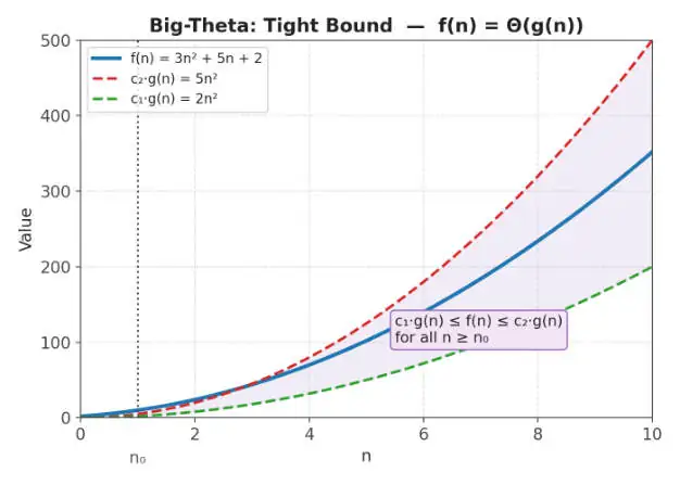
Figure 3: f(n) = 3n² + 5n + 2 is sandwiched between c₁·g(n) = 2n² and c₂·g(n) = 5n², so f(n) = Θ(n²).
Since we already proved 3n² + 5n + 2 = O(n²) and 3n² + 5n + 2 = Ω(n²) above, it immediately follows that 3n² + 5n + 2 = Θ(n²).
5.2 The Three Notations at a Glance
| Notation | Meaning | Analogy | Typical Use |
|---|---|---|---|
| O (Big-O) | Upper bound — “no slower than” | A speed limit sign: your car's speed ≤ the limit | Describing worst-case time complexity |
| Ω (Big-Omega) | Lower bound — “no faster than” | A minimum spending requirement at a store | Describing best-case or a problem's inherent lower bound |
| Θ (Big-Theta) | Tight bound — “exactly this rate” | A speedometer reading pinned within a narrow range | Describing average-case / precise growth rate |
6. Little-o and Little-omega (Brief Overview)
While Big-O, Big-Omega, and Big-Theta allow f(n) and g(n) to grow at the same rate, little-o and little-omega express strict (non-tight) bounds — useful in more advanced algorithmic analysis and complexity theory.
- f(n) = o(g(n)) (“little-o”): f(n) grows strictly slower than g(n); formally, for every constant c > 0, there exists n₀ such that f(n) < c·g(n) for all n ≥ n₀. Example: n = o(n²).
- f(n) = ω(g(n)) (“little-omega”): f(n) grows strictly faster than g(n); formally, for every constant c > 0, there exists n₀ such that f(n) > c·g(n) for all n ≥ n₀. Example: n² = ω(n).
A useful distinction: Big-O is like “≤” (less than or equal to), while little-o is like “<” (strictly less than) when comparing growth rates. Similarly, Big-Omega is like “≥”, and little-omega is like “>”.
7. Common Complexity Classes
| Notation | Name | Example Algorithm | n = 10 | n = 1,000 |
|---|---|---|---|---|
| O(1) | Constant | Accessing an array element by index | 1 op | 1 op |
| O(log n) | Logarithmic | Binary Search | ~3 ops | ~10 ops |
| O(n) | Linear | Linear Search, single loop | 10 ops | 1,000 ops |
| O(n log n) | Linearithmic | Merge Sort, Heap Sort | ~33 ops | ~10,000 ops |
| O(n²) | Quadratic | Bubble Sort, Insertion Sort, nested loops | 100 ops | 1,000,000 ops |
| O(2ⁿ) | Exponential | Naive recursive Fibonacci, subset generation | 1,024 ops | astronomically large |
| O(n!) | Factorial | Brute-force Travelling Salesman Problem | 3,628,800 ops | incomputable |
Key takeaway from the table: for small n, the difference between complexity classes may seem irrelevant, but as n scales to real-world sizes (thousands, millions), the gap becomes the difference between a program that finishes in milliseconds and one that would not finish before the heat death of the universe.
8. Rules for Deriving Time Complexity
8.1 The Sum Rule
If two blocks of code run one after another (sequentially), their complexities add: if the first block is O(f(n)) and the second is O(g(n)), the combined complexity is O(f(n) + g(n)) = O(max(f(n), g(n))). The larger term dominates.
for i in range(n): # O(n)
process(i)
for j in range(n): # O(n)
for k in range(n):
process(j, k) # O(n^2) total for this block
# Combined complexity = O(n) + O(n^2) = O(n^2) (n^2 dominates n)
8.2 The Product Rule
If a block of code is nested inside another (loop inside a loop), their complexities multiply: an outer loop running O(f(n)) times, each containing an inner block that runs O(g(n)), gives total complexity O(f(n) × g(n)).
for i in range(n): # runs n times for j in range(n): # runs n times for EACH i print(i, j) # O(1) work per iteration
# Total = O(n) * O(n) = O(n^2)
8.3 Dropping Constants and Lower-Order Terms Since asymptotic notation describes growth as n → ∞, constant multipliers and lower-order additive terms become insignificant and are dropped:
- O(5n) simplifies to O(n) — constant factors are dropped.
- O(n² + n + 100) simplifies to O(n²) — lower-order terms and constants are dropped, since n² dominates for large n.
- O(n + log n) simplifies to O(n) — since n grows faster than log n.
9. Analyzing Real Code Fragments
9.1 Example: Single Loop — O(n)
def sum_array(arr):
total = 0 for x in arr: # loop runs n times total += x # O(1) per iteration return total
# Time Complexity: O(n)
9.2 Example: Nested Loop — O(n²)
def has_duplicate(arr):
n = len(arr)
for i in range(n): # n iterations for j in range(i+1, n): # up to n iterations if arr[i] == arr[j]:
return True return False
# Time Complexity: O(n^2) -- classic quadratic pairwise comparison
9.3 Example: Divide and Conquer — O(log n)
def binary_search(arr, target, low, high):
if low > high:
return -1 mid = (low + high) // 2 if arr[mid] == target:
return mid elif arr[mid] < target:
return binary_search(arr, target, mid+1, high)
else:
return binary_search(arr, target, low, mid-1)
# Each call halves the search space: T(n) = T(n/2) + O(1) => O(log n)
9.4 Example: Recursive Fibonacci — O(2ⁿ)
def fib(n):
if n <= 1:
return n return fib(n-1) + fib(n-2)
T(n) = T(n-1) + T(n-2) + O(1) -- branches roughly double at each level
# Time Complexity: O(2^n) -- exponential, extremely inefficient for large n
10. Case Studies: Asymptotic Analysis in Practice
Case Study 1: Linear Search vs. Binary Search in a Contacts App
Imagine a phone contacts app with 100,000 saved contacts, and the user searches for a name.
- Linear Search scans every contact one by one until a match is found: worst case O(n) = 100,000 comparisons.
- Binary Search, applied on a contact list pre-sorted alphabetically, repeatedly halves the search space: worst case O(log n) ≈ 17 comparisons.
This is why every real contacts/address-book application keeps names sorted — it trades a one-time O(n log n) sorting cost for a dramatic, repeated search-time saving on every subsequent lookup, illustrating how algorithmic choice driven by asymptotic analysis directly shapes real UI responsiveness.
Case Study 2: Bubble Sort vs. Merge Sort at Internet Scale
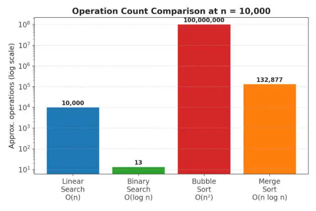
Figure 4: Approximate operation counts at n = 10,000 (log scale) — note how dramatically O(n²) diverges from O(n log n).
A company like an e-commerce platform sorting a product catalog of n = 10,000 items would need roughly 100,000,000 comparisons using Bubble Sort's O(n²) behavior, versus roughly 132,877 comparisons using Merge Sort's O(n log n) behavior — a difference of nearly three orders of magnitude. At the scale of Amazon or Flipkart, with catalogs of tens of millions of products, an O(n²) sorting algorithm would be computationally infeasible, which is exactly why production database engines and standard libraries use O(n log n) algorithms (Timsort, Merge Sort, Quicksort with good pivots) internally.
Case Study 3: Google Maps / GPS Routing and Graph Algorithms
Finding the shortest driving route between two points uses Dijkstra's algorithm, whose time complexity with a binary-heap-based priority queue is O((V + E) log V), where V is the number of road intersections (vertices) and E is the number of road segments (edges). Understanding this asymptotic bound is what allows engineers to
predict that, even for a road network graph with millions of nodes (e.g., an entire country), the algorithm remains tractable — in contrast to a naive brute-force approach that checks every possible path, which would be O(V!) and utterly infeasible.
Case Study 4: Why Comparison-Based Sorting Cannot Beat O(n log n)
This is a classic application of Big-Omega. It can be proven (using a decision-tree argument over all n! possible orderings of n elements) that any comparison-based sorting algorithm requires Ω(n log n) comparisons in the worst case. This lower bound explains why Merge Sort and Heap Sort, which achieve O(n log n), are considered asymptotically optimal comparison-based sorting algorithms — no comparison-based algorithm can ever do fundamentally better, no matter how cleverly it is written.
11. Common Misconceptions and Pitfalls
- “O(n) always means the algorithm is fast.” — Not necessarily; the hidden constant matters for small/medium n. O(n) with a huge constant factor can be slower in practice than O(n²) with a tiny constant, for small inputs. Asymptotic notation only describes behavior as n → ∞.
- “Big-O always describes the worst case.” — Big-O describes an upper bound on any case (best, worst, or average) you choose to analyze; it is commonly applied to worst-case analysis by convention, but it is not exclusively a worst-case notation.
- “O(n²) and Θ(n²) mean the same thing.” — O(n²) only claims an upper bound (the function could actually grow slower, e.g., O(n) functions are technically also O(n²)); Θ(n²) is a precise, tight claim that the function grows at exactly the rate of n².
- Forgetting to drop constants/lower-order terms, e.g., writing O(2n² + 3n) instead of the correctly simplified O(n²).
12. Practice Questions for Students (with Answers)
Q1. Define Big-O notation formally and explain what it guarantees about an algorithm.
Answer: f(n) = O(g(n)) if there exist positive constants c and n₀ such that 0 ≤ f(n) ≤ c·g(n) for all n ≥ n₀. It guarantees an upper bound: the algorithm's running time will never grow faster than a constant multiple of g(n) once the input is large enough. It does not claim this bound is the tightest possible.
Q2. Prove that 5n + 3 = O(n).
Answer: We need constants c, n₀ such that 5n + 3 ≤ c·n for all n ≥ n₀. For n ≥ 1, 3 ≤ 3n, so 5n + 3 ≤ 5n + 3n = 8n. Choosing c = 8 and n₀ = 1 satisfies the definition. Hence 5n + 3 = O(n). ■
Q3. What is the time complexity of two sequential loops, one running n times and the other running n² times? Explain using the sum rule.
Answer: By the sum rule, sequential blocks add their complexities: O(n) + O(n²) = O(n + n²). Since n² dominates n for large n, this simplifies to O(n²).
Q4. Why is Big-Omega useful for describing the inherent difficulty of a problem, using comparison-based sorting as an example?
Answer: Big-Omega establishes a lower bound that applies to every possible algorithm solving a problem, not just one specific implementation. For comparison-based sorting, it has been proven that Ω(n log n) comparisons
are required in the worst case for ANY comparison-based algorithm, meaning no future cleverer algorithm using only comparisons can ever beat this bound — it is a fundamental property of the problem itself, not a weakness of a specific algorithm.
Q5. Differentiate Big-O and Big-Theta with an example where a function is O(n²) but NOT Θ(n²).
Answer: Big-O gives only an upper bound, while Big-Theta gives a tight (upper and lower) bound. The function f(n) = n is O(n²) (since n ≤ c·n² for appropriate c and n₀), but f(n) = n is NOT Θ(n²), because n does not also satisfy the lower bound c₁·n² ≤ n for large n (n grows strictly slower than n²).
Q6. What is the time complexity of the following code, and why?
for i in range(n):
j = 1 while j < n:
j = j * 2
# O(1) work
Answer: The outer loop runs n times. The inner while loop doubles j each iteration, so it runs O(log n) times before j ≥ n. By the product rule, total complexity = O(n) × O(log n) = O(n log n).
13. Interview-Style Questions (with Answers)
Q1. Why do interviewers care about time complexity when evaluating a candidate's solution, even if the code runs correctly and fast on the given test cases?
Answer: Small test cases can hide inefficiency — an O(n²) solution may pass instantly on n = 100 but time out or crash in production on n = 10,000,000. Interviewers assess asymptotic complexity to judge whether a candidate's solution will scale to real-world data sizes, and whether the candidate understands the trade-offs (e.g., time vs. space) behind their chosen approach, not just whether it works for the sample input.
Q2. You're asked to find whether an array contains a pair of elements that sum to a target value. Compare a brute-force O(n²) approach with an O(n) hash-set-based approach.
Answer: The brute-force approach checks every pair using nested loops — O(n²) time, O(1) extra space. The optimized approach iterates once through the array, and for each element x, checks whether (target - x) already exists in a hash set built so far, inserting x into the set afterward — O(n) time due to O(1) average-case hash set lookups, at the cost of O(n) extra space. This demonstrates the classic time-space trade-off central to algorithm design interviews.
Q3. What is amortized time complexity, and how does it differ from worst-case time complexity? Give an example.
Answer: Amortized complexity averages the cost of an operation over a sequence of operations, rather than analyzing a single operation in isolation. For example, appending to a dynamic array (like Python's list or Java's ArrayList) is usually O(1), but occasionally triggers an O(n) resize/copy operation when capacity is exceeded. Even though a single append can be O(n) in the worst case, the amortized cost over n appends is O(1) per operation, because the expensive resizes happen rarely enough (doubling strategy) that their cost, spread across all operations, averages out to a constant.
Q4. Two algorithms solve the same problem: Algorithm A is O(n log n) and Algorithm B is O(n²), but B has a much smaller constant factor. When might you actually prefer Algorithm B in a real system?
Answer: For small or bounded input sizes (a known upper limit on n, e.g., sorting a UI list capped at 50 items), the lower constant factor of Algorithm B may make it faster in absolute wall-clock time despite its worse asymptotic growth. Many real-world library implementations (e.g., Timsort, Introsort) even switch to a simple O(n²) algorithm like Insertion Sort for small sub-arrays because its low overhead outperforms O(n log n) algorithms below a certain size threshold. This illustrates that asymptotic notation guides design but must be balanced with practical, empirical benchmarking.
Q5. How would you explain the difference between O(n) and O(log n) to a non-technical stakeholder, using an analogy?
Answer: An O(n) search is like looking for a name in an unsorted phonebook by checking every page one at a time from the start. An O(log n) search is like looking for a name in a sorted phonebook by always opening to the middle, deciding whether to go left or right based on alphabetical order, and repeating — each step eliminates half of the remaining pages, so even a phonebook with a million entries can be searched in about 20 steps instead of up to a million.
14. Summary and Key Takeaways
- Asymptotic notation abstracts away hardware, language, and constant-factor differences to compare algorithms purely by how their resource usage scales with input size n.
- Big-O (O) gives an upper bound (“no worse than”), Big-Omega (Ω) gives a lower bound (“no better than”), and Big-Theta (Θ) gives a tight bound (“exactly this rate”).
- Little-o and little-omega express strict (non-tight) versions of these bounds, used in more formal complexity analysis.
- The sum rule (sequential code adds complexities, larger term dominates) and the product rule (nested code multiplies complexities) are the two workhorse tools for analyzing real code.
- Constants and lower-order terms are always dropped in the final simplified notation.
- Real systems — contact search apps, e-commerce catalogs, GPS navigation — are all engineered around these growth-rate trade-offs, making asymptotic analysis one of the most practically important tools in a computer scientist's toolkit.
“Premature optimization is the root of all evil — but so is ignoring asymptotic complexity until it's too late.” A well-trained engineer knows the Big-O of their code before they know its exact runtime in milliseconds.